Statistiek I

• Non-parametric tests:
  • Mann-Whitney U test (alternative to independent samples \(t\)-test)
  • Wilcoxon signed-rank test (alternative to paired and single sample \(t\)-test)
  • Sign test (alternative to Wilcoxon signed-rank test)
• Reporting statistical analysis

• \(p\)-value: probability of the observed (or more extreme) data given that \(H_0\) true
  • Two-tailed test: very low and very high values evidence against \(H_0\)
  • One-tailed test: only low (or high) values evidence against \(H_0\)
• In R: parameter alternative="two-tailed" yields \(p\)-value for two-tailed test
  • alternative="less" (or "greater"): \(p\)-value for one-tailed test
  • (No need to divide/multiply by 2, in contrast to using pnorm() or pt())
  • \(p\)-value of a one-tailed test (appropriate side) will be half of \(p\)-value of two-tailed test (due to symmetry)
• \(p\)-value is compared to the \(\alpha\)-value (set before analysis)
  • One-tailed test (on appropriate side) is more likely to yield significant result (as \(p\)-value is lower)

• Assessing the relationship between variables of the same type
  • Two categorical variables: \(\chi^2\)-test and Fisher’s exact test
  • Two numerical variables: Pearson correlation
• Reliability of questionnaires: Cronbach’s \(\alpha\)

• RQ: Is there a different influence of BAC on L1 vs. L2 language proficiency?
  • Note: not conclusively answered in this course (regression necessary: Statistiek II)
• BAC and L1 and L2 speech samples collected for about 90 native Dutch speakers
• Dutch speech samples were rated by native Dutch speakers (at Lowlands)
• English speech samples were rated by native American English speakers (online)
• For each speaker, the ratings were averaged per language
• Other variables we collected included sex, education level, drug use, etc.
  • Relationships between these variables will be looked at in this lecture
  • First: sex and alcohol use (BAC > 0 vs. BAC = 0)

• In earlier lectures, we were interested in the relationship between a categorical variable (two groups) and a numerical variable (e.g., English grades)
• But what about the relationship between two categorical variables?
• Examples:
  • Social group and /r/ pronunciation
  • Authorship and use of personal pronouns
  • Biological sex and drinking alcohol or not

(counts <- table(llsNL$sex, llsNL$alcohol))

#         
#          Alcohol No-alcohol
#   Female      21         31
#   Male        26         13

prop.table(counts)  # as proportions

#         
#          Alcohol No-alcohol
#   Female 0.23077    0.34066
#   Male   0.28571    0.14286

prop.table(counts, 1)  # proportions per row

#         
#          Alcohol No-alcohol
#   Female 0.40385    0.59615
#   Male   0.66667    0.33333

prop.table(counts, 2)  # proportions per column

#         
#          Alcohol No-alcohol
#   Female 0.44681    0.70455
#   Male   0.55319    0.29545

barplot(counts, legend = c("F", "M"), beside = T, ylim = c(0, 60), main = "Beside")
barplot(counts, legend = c("F", "M"), ylim = c(0, 60), main = "Segmented")

plot of chunk unnamed-chunk-4

• $\chi^2$-test is used for assessing the relationship between two categorical variables
  • Is the distribution of one variable affected by the distribution of another?
    • \(P(A|B) \neq P(A)\)?
    • Example: \(P(\textrm{having had alcohol}|\textrm{sex = M}) \neq P(\textrm{having had alcohol})\)?
  • We can test this by counting

• The $\chi^2$-test compares the actual frequencies to the expected frequencies (assuming that the two variables are unrelated, i.e. independent)
  • Large differences: likely related
  • Small differences: most likely not related
• Note: not for paired data (i.e. repeated measures for one individual)!
  • Then the McNemar test is appropriate (not covered in this course)

• Data randomly selected from population
• Independent observations
• Each observation can be classified into exactly one category per variable
• Expected frequency in each cell \(\geq\) 5
  • Otherwise we use Fisher’s exact test (covered later this lecture)

• Actual frequencies (including column and row sums)

• Expected frequencies: multiply column total with row proportions

$$\chi^2 = \Sigma \frac{(O - E)^2}{E}$$

• \(\chi^2\) = 1.28 + 1.36 + 1.7 + 1.82 \(\approx\) 6.16
• Degrees of freedom: (R - 1) \(\times\) (C - 1) = (2 - 1) \(\times\) (2 - 1) = 1
  • With R: number of rows, C: number of columns
  • If row and column totals are known together with (R - 1) \(\times\) (C -1) values, all other values can be calculated

• \(p\)-value associated with \(\chi^2\) value is dependent on the shape of the distribution
• Shape of the \(\chi^2\) distribution is dependent on number of degrees of freedom (dF)

plot of chunk unnamed-chunk-8

chisq.test(counts, correct = FALSE)  # chi-square test, no continuity correction

# 
# 	Pearson's Chi-squared test
# 
# data:  counts
# X-squared = 6.16, df = 1, p-value = 0.013

• Using an \(\alpha\)-level of 0.05, this association (biological sex and alcohol use) is significant
• Note that we always set correct = FALSE, as using Yates’ correction is not recommended (lowers dF: too conservative)

• Flexible measure for effect size of the relation between two variables: Cramer’s \(V\)
  • Cramer’s \(V\): scaled \(\chi^2\) value (between 0 and 1)
  • Negligible: \(V < 0.1\), small: \(V < 0.3\), medium: \(V < 0.5\), large: \(V \geq 0.5\)
    (for tables with 2 rows or 2 columns)
• Another measure of effect size is the odds ratio: see Levshina, p. 208

library(vcd)  # install with: install.packages('vcd')
assocstats(counts)

#                     X^2 df P(> X^2)
# Likelihood Ratio 6.2536  1 0.012394
# Pearson          6.1642  1 0.013036
# 
# Phi-Coefficient   : 0.26 
# Contingency Coeff.: 0.252 
# Cramer's V        : 0.26

• The effect size for the relation between alcohol use and biological sex is small

• Are biological sex and having had (soft or hard) drugs related?

(counts <- table(llsNL$sex, llsNL$drugs))  # actual frequencies

#         
#          No Soft Hard
#   Female 49    1    2
#   Male   37    1    1

chisq.test(counts)$expected  # expected frequencies

#         
#              No    Soft   Hard
#   Female 49.143 1.14286 1.7143
#   Male   36.857 0.85714 1.2857

• The \(\chi^2\)-test will give a warning with expected frequencies < 5

chisq.test(counts, correct = F)

# Warning in chisq.test(counts, correct = F): Chi-squared approximation may be
# incorrect

# 
# 	Pearson's Chi-squared test
# 
# data:  counts
# X-squared = 0.154, df = 2, p-value = 0.93

• In this course, we use Fisher’s exact test when low expected frequencies occur
  • But note that it is conservative, and alternatives exist (e.g., Fisher-Boschloo test)

fisher.test(counts)

# 
# 	Fisher's Exact Test for Count Data
# 
# data:  counts
# p-value = 1
# alternative hypothesis: two.sided

assocstats(counts)

#                      X^2 df P(> X^2)
# Likelihood Ratio 0.15618  2  0.92488
# Pearson          0.15375  2  0.92601
# 
# Phi-Coefficient   : NA 
# Contingency Coeff.: 0.041 
# Cramer's V        : 0.041

• The effect size for the relation between having had drugs and biological sex is negligible

• We are interested in assessing whether sex and education level are significantly (with \(\alpha\) = 0.05) related (i.e. dependent)
• Hypotheses:
  • \(H_0\): sex and education level are independent
  • \(H_a\): sex and education level are dependent

(counts <- table(llsNL$sex, llsNL$edu))

#         
#          PVMBO HBO WO
#   Female    10   9 33
#   Male      10  14 15

• Data randomly selected from population ?
• Independent observations ✓
• Each observation can be classified into exactly one category per variable ✓
• Expected frequency in each cell \(\geq\) 5 ?

round(chisq.test(counts)$expected)

#         
#          PVMBO HBO WO
#   Female    11  13 27
#   Male       9  10 21

• All expected frequencies \(\geq\) 5: ✓

barplot(counts, legend = c("F", "M"), col = c("pink", "lightblue"), ylim = c(0, 70))

plot of chunk unnamed-chunk-17

chisq.test(counts, correct = F)

# 
# 	Pearson's Chi-squared test
# 
# data:  counts
# X-squared = 6.1, df = 2, p-value = 0.047

• \(p\)-value < \(\alpha\)-value: reject \(H_0\) and accept \(H_a\)

assocstats(counts)

#                     X^2 df P(> X^2)
# Likelihood Ratio 6.1500  2 0.046189
# Pearson          6.1044  2 0.047255
# 
# Phi-Coefficient   : NA 
# Contingency Coeff.: 0.251 
# Cramer's V        : 0.259

• The effect size is small

chisq.test(counts)$expected  # expected frequencies

#         
#            PVMBO     HBO     WO
#   Female 11.4286 13.1429 27.429
#   Male    8.5714  9.8571 20.571

chisq.test(counts)$observed  # observed frequencies

#         
#          PVMBO HBO WO
#   Female    10   9 33
#   Male      10  14 15

prop.table(counts, 2)  # column proportions (2nd index)

#         
#          PVMBO  HBO   WO
#   Female  0.50 0.39 0.69
#   Male    0.50 0.61 0.31

prop.table(counts, 1)  # row proportions (1st index)

#         
#          PVMBO  HBO   WO
#   Female  0.19 0.17 0.63
#   Male    0.26 0.36 0.38

• Standardized residuals: \(z\)-scores indicating where the largest differences are
  • (Standardization against expected frequency and row and column proportion)
  • Only useful when one of the variables has > 2 levels: otherwise |values| equal

chisq.test(counts)$stdres  # z-scored differences

#         
#             PVMBO      HBO       WO
#   Female -0.73078 -2.01934  2.36396
#   Male    0.73078  2.01934 -2.36396

• The WO education level shows the largest deviation from the expected sex distribution

We tested whether sex (two levels: male and female) and education level (three levels: PVMBO, HBO and WO) were related (with \(\alpha\) = 0.05). Our hypotheses were \(H_0\): sex and education level are independent, and \(H_a\): sex and education level are dependent. In our sample of 91 participants from the Lowlands Science experiment, we obtained the participants’ sex and education level. Table 1 shows their relation and Figure 1 shows a bar plot visualizing the results of the table. As both variables are nominal, and the expected frequency of each combination was greater than 5, we assessed the dependence of the two variables using the \(\chi^2\) test: \(\chi^2(2) = 6.1\), \(p = 0.047\). As the \(p\)-value was lower than the \(\alpha\)-level, the result was significant. We reject the null hypothesis and accept the alternative hypothesis that sex and education level are dependent. The difference from the expected distribution was greatest for the WO group: there were many more females than expected. The effect size was small (Cramer’s \(V\) = 0.26).

• Avoid overuse of \(\chi^2\):
  • When tables have very large frequencies (e.g., corpus linguistics) results are almost always significant
• \(\chi^2\) is not very sensitive, so use numerical variables where appropriate
  • I.e. don’t use: This course was: useless / somewhat useful / useful
  • But use Likert scales:
    • On a scale from 1-5, this course was: … (1: useless; 5: useful)

• Patient survival after surgery:

• With the original information, Hospital B appears better
• But consider:

• Hospital A is better in both categories!
  • But it attracts more difficult patients (perhaps because it’s better), so its overall survival rate is lower

• Simpson’s Paradox: the distribution of a nominal variable can be reversed under aggregation
  • This is caused by hidden variables, variables which are important, but neglected in the analysis

• In contrast to two nominal variables, it is much easier to assess the relationship between two numerical variables
• We can visualize such a relationship in a scatter plot

plot(llsNL$BAC, llsNL$rating)

plot of chunk unnamed-chunk-26

• We can quantify the relationship between two variables \(x\) and \(y\) by calculating the Pearson correlation coefficient \(r\)
• After standardizing (i.e. converting the values of each variable to \(z\)-scores), we can calculate the correlation between \(z_x\) and \(z_y\): $$r = \frac{1}{n-1} \sum_{i=1}^{n} z_{x_i} z_{y_i}$$
• Note: division by \(n-1\) to match with the \(n-1\) in formula for sample standard deviation (used in \(z\)-score calculation)
• Values range between \(-1 \leq r \leq 1\): strength and direction of the effect

sum( scale(llsNL$BAC) * scale(llsNL$rating) ) / ( nrow(llsNL) - 1 ) # manual

# [1] -0.34045

cor(llsNL$BAC, llsNL$rating) # using the cor function (easier)

# [1] -0.34045

cor(llsNL$BAC, llsNL$rating)  # when speaking Dutch

# [1] -0.34045

cor(llsEN$BAC, llsEN$rating)  # when speaking English

# [1] -0.11235

• With NA values, parameter use needs to be set to "pairwise.complete.obs"

llsNL[1, ]$rating = NA  # set 1 value to NA (only for illustration)
cor(llsNL$BAC, llsNL$rating)  # will result in NA 

# [1] NA

cor(llsNL$BAC, llsNL$rating, use = "pairwise.complete.obs")

# [1] -0.36322

• Shoe size and reading ability are correlated
• Is there a dependency between the two?
• No: the hidden variable age affects both shoe size and reading ability!
• Experiments are necessary to control for potential causes (and confounding factors)

• In this course, we are not assessing whether a correlation is statistically significant
  • But it is possible: function cor.test() conducts this test
    • However, there are several required assumptions (see Levshina 6.2.3)
  • Or you can use regression: covered in Statistiek II
  • Non-parametric alternatives to the correlation are also available
    • For example: Spearman’s \(\rho\) (correlation of ranks, see Levshina 6.3)

• Questionnaires are an easy way to obtain much data
• But: how to ask the right question?
• For example: How do students feel about statistics?
  • What type of statistics?
  • What kind of feelings?
• For this reason, researchers ask several questions all aimed at acquiring similar information (i.e. questions are combined in a so-called scale)

• Validity: are you measuring what you intend to measure?
  • This can be checked by consulting experts, comparing to similar measures, etc.
• Reliability: is your measure consistent?
  • I.e. are results repeatable when obtained given the same conditions?
  • This can be statistically assessed using Cronbach’s \(\alpha\)
• Reliability \(\neq\) validity!

• Underlying idea:
  • If we split the questions, how well do two halves of the questionnaire agree?
  • And if there are many questions, how well would they agree if we looked at all possible ways of splitting?
• More information: https://www.ijme.net/archive/2/cronbachs-alpha.pdf

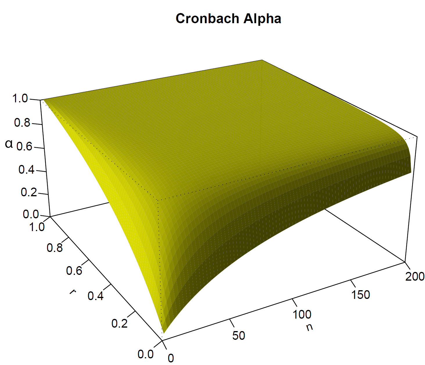
• Cronbach’s \(\alpha\) depends on:
  • The average correlation of all variables (i.e. questions) involved
  • The number of questions
• Removing a problematic question may increase Cronbach’s \(\alpha\)
• Cronbach’s \(\alpha\): > 0.7 is acceptable, 0.8 is good, 0.9 is very good
  • With Cronbach’s \(\alpha\) > 0.7: mean of items can be used as summary of the scale

• Questions (in English): https://goo.gl/efxtre

load("sats.rda")
head(sats)  # scores 1-7: negative - positive (some inverted)

#   Q3 Q4 Q14 Q15 Q18 Q19 Q28
# 1  7  2   6   2   2   6   1
# 2  4  4   3   4   4   4   4
# 3  3  3   6   6   5   2   6
# 4  5  4   6   4   3   6   2
# 5  4  5   6   4   4   2   5
# 6  4  2   6   2   3   5   2

• Note that I have included one question which is part of a different scale
  • We will try to identify this question later

library(psych)
result <- alpha(sats)

# Some items ( Q3 Q19 ) were negatively correlated with the first principal component and 
# probably should be reversed.  
# To do this, run the function again with the 'check.keys=TRUE' option

summary(result)

# 
# Reliability analysis   
#  raw_alpha std.alpha G6(smc) average_r  S/N   ase mean   sd median_r
#       0.41      0.37    0.63     0.078 0.59 0.039  4.2 0.69    0.042

• Reliability is very low, but we ignored some questions having an inverted scale

• The instructions of the questionnaire show that questions 4, 15, 18 and 28 should be inverted (1 \(\rightarrow\) 7, 2 \(\rightarrow\) 6, 3 \(\rightarrow\) 5, 4 \(\rightarrow\) 4, etc.)

result <- alpha(sats, keys = c("Q4", "Q15", "Q18", "Q28"))  # keys: scales inverted
summary(result)  # much better reliability

# 
# Reliability analysis   
#  raw_alpha std.alpha G6(smc) average_r S/N   ase mean   sd median_r
#       0.79      0.75    0.81       0.3   3 0.013  4.3 0.98     0.36

result$alpha.drop

#      raw_alpha std.alpha G6(smc) average_r  S/N alpha se var.r med.r
# Q3        0.74      0.69    0.73      0.27 2.18     0.02  0.10  0.36
# Q4-       0.74      0.70    0.76      0.28 2.29     0.02  0.09  0.37
# Q14       0.84      0.84    0.85      0.46 5.10     0.01  0.02  0.38
# Q15-      0.77      0.73    0.80      0.31 2.67     0.01  0.12  0.37
# Q18-      0.73      0.69    0.75      0.27 2.18     0.02  0.09  0.35
# Q19       0.75      0.69    0.73      0.27 2.21     0.02  0.10  0.35
# Q28-      0.71      0.67    0.73      0.26 2.06     0.02  0.08  0.35

• Dropping Q14 would yield a higher Cronbach’s \(\alpha\)

sats2 <- sats[, -3]  # drop third column (Q14)
result2 <- alpha(sats2, keys = c("Q4", "Q15", "Q18", "Q28"))  # keys: scales inverted
summary(result2)

# 
# Reliability analysis   
#  raw_alpha std.alpha G6(smc) average_r S/N   ase mean  sd median_r
#       0.84      0.84    0.85      0.46 5.1 0.011    4 1.2     0.38

• In this lecture, we’ve covered:
  • \(\chi^2\)-test for assessing relationship between 2 nominal variables
  • Pearson correlation for assessing relationship between 2 numerical variables
  • Cronbach’s \(\alpha\) for assessing reliability of multiple numerical variables
  • Hidden variables
  • A (cor)relation does not imply causation
  • Reliability is no validity
• Experiment with correlation: https://eolomea.let.rug.nl/Statistiek-I/HC6
• Next lecture: practice exam
• (We run many experiments and outreach events in our lab, for example using our SPRAAKLAB mobile laboratory; get in contact if you would like to get involved!)