load('dat.rda')
head(dat)Basic statistical tests
Martijn Wieling (University of Groningen)
This lecture
- Dataset for this lecture
- Comparing one or two groups: \(t\)-test
- Non-parametric alternatives: Mann-Whitney U and Wilcoxon signed rank
- Assessing the dependency between two categorical variables: \(\chi^2\) test
- Comparing more than two groups: ANOVA
Some basic points
- This lecture focuses on how-to-use and when-to-use, rather than on the underlying calculations
- Make sure to report effect size as significance is dependent on sample size
| difference (in \(s\)) | \(n\) | \(p\) |
|---|---|---|
| 0.01 | 40,000 | 0.05 |
| 0.10 | 400 | 0.05 |
| 0.25 | 64 | 0.05 |
| 0.54 | 16 | 0.05 |
Question 1
Dataset for this lecture
   Speaker Language  PronDist PronDistCat LangDist LangDistAlt Age Sex AEO LR NrLang
1  arabic1   arabic  0.185727   Different  0.63699     0.44864  38   F  12  4      0
2 arabic10   arabic -0.172175     Similar  0.63699     0.44864  26   M   5  2      2
3 arabic13   arabic -0.035423     Similar  0.63699     0.44864  25   M  15  1      2
4 arabic12   arabic  0.372547   Different  0.63699     0.44864  32   M  11  8      0
5 arabic17   arabic -0.175237     Similar  0.63699     0.44864  35   M  15  0      1
6 arabic18   arabic  0.168120   Different  0.63699     0.44864  18   M   6  0      1
Dataset structure
'data.frame':   712 obs. of  11 variables:
 $ Speaker    : Factor w/ 712 levels "afrikaans1","afrikaans2",..: 21 22 25 24 27 28 26 30 31 23 ...
 $ Language   : Factor w/ 159 levels "afrikaans","agni",..: 7 7 7 7 7 7 7 7 7 7 ...
 $ PronDist   : num  0.1857 -0.1722 -0.0354 0.3725 -0.1752 ...
 $ PronDistCat: Factor w/ 2 levels "Different","Similar": 1 2 2 1 2 1 1 2 2 2 ...
 $ LangDist   : num  0.637 0.637 0.637 0.637 0.637 ...
 $ LangDistAlt: num  0.449 0.449 0.449 0.449 0.449 ...
 $ Age        : num  38 26 25 32 35 18 22 36 23 30 ...
 $ Sex        : Factor w/ 2 levels "F","M": 1 2 2 2 2 2 2 2 1 1 ...
 $ AEO        : num  12 5 15 11 15 6 16 12 10 14 ...
 $ LR         : num  4 2 1 8 0 0 0 1 0 4 ...
 $ NrLang     : int  0 2 2 0 1 1 2 2 2 1 ...
Comparing one or two groups: \(t\)-test
- Values between two groups (or vs. value) can be compared using the \(t\)-test
- Assumptions:
- Randomly selected sample(s)
- Independent observations (except for paired data)
- Data has interval scale (difference between two values is meaningful) or ratio scale (meaningful difference and true 0)
- E.g., interval scale: temperature in C; ratio scale: length in cm.
- Data in sample(s) normally distributed (for \(N \leq 30\))
- Variances in samples homogeneous (Welch’s adjustment, default in
R, corrects for this) - Note: Likert scale is ordinal data, so \(t\)-test in principle not adequate
- But in practice not problematic (De Winter & Dodou, 2011)
- Visualize the data if possible (facilitates interpretation)
Question 2
\(t\)-test
- Result of \(t\)-test is a \(t\)-value, which is compared to the appropriate \(t\)-distribution
- \(t\)-distribution depends on degrees of freedom (therefore: report dF!)

Group mean vs. value: visualization

Group mean vs. value: one sample \(t\)-test
One sample \(t\)-test: effect size
- Cohen’s \(d\) measures the difference in terms of the number of standard deviations
- Rough guideline: Cohen’s \(d\) < 0.3: small effect size; 0.3 - 0.8: medium; > 0.8: large
Try it yourself!
- Install the Mathematical Biostatistics Boot Camp swirl course:
- Run
swirl()in RStudio and finish the following lesson of the Mathematical Biostatistics Boot Camp course:- Lesson 1: One Sample t-test
Comparing paired data: visualization

Paired samples \(t\)-test
    Paired t-test

data:  lang$LangDist and lang$LangDistAlt
t = -3.73, df = 158, p-value = 0.00027
alternative hypothesis: true mean difference is not equal to 0
95 percent confidence interval:
 -0.085703 -0.026367
sample estimates:
mean difference
      -0.056035
Question 3
Paired samples \(t\)-test = one sample \(t\)-test
    One Sample t-test

data:  lang$LangDist - lang$LangDistAlt
t = -3.73, df = 158, p-value = 0.00027
alternative hypothesis: true mean is not equal to 0
95 percent confidence interval:
 -0.085703 -0.026367
sample estimates:
mean of x
-0.056035 [1] 0.29585Comparing two groups: visualization

Comparing two groups: independent samples \(t\)-test
    Welch Two Sample t-test

data:  PronDist by Language
t = -3.56, df = 42.5, p-value = 0.00092
alternative hypothesis: true difference in means between group german and group russian is not equal to 0
95 percent confidence interval:
 -0.267719 -0.074108
sample estimates:
 mean in group german mean in group russian
-0.150222 0.020691 [1] 1.0166Reporting results of a \(t\)-test
Pronunciation difference from native English was smaller for the German speakers (mean: \(-0.15\), sd: \(0.132\)) than for the Russian speakers (mean: \(0.02\), sd: \(0.194\)). The difference was \(-0.17\) (Cohen’s \(d\): \(1.02\), large effect) and reached significance using an independent samples Welch’s unequal variances \(t\)-test at an \(\alpha\)-level of \(0.05\), \(t(42.5) = -3.56, p < 0.001\).
Assumptions met?
- ✓ Randomly selected sample(s)
- ✓ Independent observations (except for pairs)
- ✓ Data has interval or ratio scale
- ? Variance in samples homogeneous (corrected with Welch’s adjustment)
- ? Data in compared samples are normally distributed (for \(N \leq 30\))
Testing if variances are equal (homoscedasticity)
- Testing homoscedasticity using Levene’s test
Levene's Test for Homogeneity of Variance (center = median)
      Df F value Pr(>F)
group  1       5   0.03 *
      45
---
Signif. codes: 0 '***' 0.001 '**' 0.01 '*' 0.05 '.' 0.1 ' ' 1- Levene’s test shows that the variances are different and the default Welch’s adjustment is warranted
- But note that the Welch’s \(t\)-test can always be used as it is more robust and power is comparable to that of the normal \(t\)-test
Assessing normality: Russian data (1)
- For investigating normality, a normal quantile plot can be used

Assessing normality: Russian data (2)
- Alternatively, one can use the Shapiro-Wilk test of normality
Question 4
Assessing normality: German data (1)

Assessing normality: German data (2)
    Shapiro-Wilk normality test

data:  german$PronDist
W = 0.929, p-value = 0.12- Sensitivity to sample size of the Shapiro-Wilk test is clear: I would judge the data as non-normal on the basis of the normal quantile plot
- Given the small size of the sample (N = 22$), a non-parametric alternative is needed
Non-parametric alternatives
- Non-parametric fallbacks
- One sample \(t\)-test and paired \(t\)-test: Wilcoxon signed rank test
- Independent samples \(t\)-test: Mann-Whitney U test (= Wilcoxon rank sum test)
- In both cases:
wilcox.test(similar tot.test)
Comparing two groups: Mann-Whitney U test (1)

Comparing two groups: Mann-Whitney U test (2)
    Wilcoxon rank sum exact test

data:  PronDist by Language
W = 140, p-value = 0.0035
alternative hypothesis: true location shift is not equal to 0
wilcox.effsize <- function(pval2tailed, N){
( r <- abs( qnorm(pval2tailed / 2) / sqrt(N) ) ) # r = z / sqrt(N)
}
# rough guideline: r around 0.1 (small), > 0.3 (medium), > 0.5: large
wilcox.effsize(model$p.value,nrow(rusger)) [1] 0.42616Reporting results of Mann-Whitney U (or Wilcoxon)
Pronunciation difference from native English was smaller for the German speakers (median value: \(-0.16\)) than for the Russian speakers (median value: \(0.006\)). The effect size \(r\) of the difference was \(0.43\) (medium) and reached significance using a Mann-Whitney U test (\(U = 140\), with \(n_g = 22\) and \(n_r = 25\)) at an \(\alpha\)-level of \(0.05\) (\(p = 0.003\)).
Question 5
Group mean vs. value: Wilcoxon signed rank (1)

Group mean vs. value: Wilcoxon signed rank (2)
Comparing paired data: Wilcoxon signed rank

Comparing paired data: Wilcoxon signed rank
- Using a Wilcoxon signed rank test is not necessary, given the size of the dataset (159 languages) and the normal distribution, but it is included for completeness
    Wilcoxon signed rank test with continuity correction

data:  lang$LangDist and lang$LangDistAlt
V = 4362, p-value = 0.00059
alternative hypothesis: true location shift is not equal to 0[1] 0.27242Dependency between two cat. variables: \(\chi^2\) test
- Requirements:
- Sample randomly selected from the population of interest
- Independent observations
- Every observation can be classified into exactly one category
- Expected frequency for each combination at least 5 (or: Fisher’s exact test)
- Intuition: compare expected frequencies with observed frequencies
- Larger differences between expected and observed: more likely two categorical variables dependent
\(\chi^2\) test
\(\chi^2\) test: effect size
- Rough guidelines for effect size:
- Small effect: \(w = 0.1\)
- Medium effect: \(w = 0.3\)
- Large effect: \(w = 0.5\)
- With \(w = V \times \sqrt{min(R,C) - 1}\)
- With more rows (R) and columns (C), a lower Cramer’s \(V\) can still be the same size of effect
\(\chi^2\) test: reporting results
Fisher’s exact test of independence was performed to examine the relation between Language and Pronunciation Distance Category. The relation between the two variables was significant in a sample size of 31 at an \(\alpha\)-level of \(0.05\), \(\chi^2 (2) = 6.25, p = 0.04\). The effect size was medium, with Cramer’s \(V\): \(0.45\).
However, \(\chi^2\) test not appropriate: Fisher’s exact test
             farsi polish swedish
  Different 4.1935 4.6129  4.1935
  Similar   5.8065 6.3871  5.8065
Fisher's Exact Test for Count Data
data: tab
p-value = 0.053
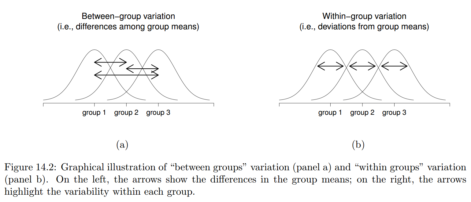
alternative hypothesis: two.sidedANOVA for differences between 3 or more groups
- Intuition of ANOVA: compare between-group variation and within-group variation
- If between-group variation (\(SS_b\): sum of squares) is large relative to within-group variation (\(SS_w\)) the difference is more likely to be significant
- See this freely downloadable, well-written statistics book
Assumptions for ANOVA
- Randomly selected sample(s)
- Independent observations in the groups
- Data has interval scale or ratio scale
- Data in each sample is normally distributed and/or equal sample sizes
- Variance in samples homogeneous
Differences between 3+ groups: one-way ANOVA (1)

Differences between 3+ groups: one-way ANOVA (2)
result <- aov(PronDist ~ Language, data=dat3)
# alternative if variances are not equal: oneway.test(),
# alternative if non-normal distribution: kruskal.test()

summary(result) # is the ANOVA significant?
Df Sum Sq Mean Sq F value Pr(>F)
Language 2 0.213 0.1067 4.16 0.026 *
Residuals 28 0.718 0.0256
---
Signif. codes: 0 '***' 0.001 '**' 0.01 '*' 0.05 '.' 0.1 ' ' 1 eta.sq eta.sq.part
Language 0.22908 0.22908Question 6
ANOVA: reporting results
At an \(\alpha\)-level of \(0.05\), a one-way ANOVA showed a significant effect of Language on Pronunciation Difference from English: \(F(2,28) = 4.16\) (\(p = 0.03\)). The effect size of Language, partial eta squared \(\eta^2_p\), was equal to \(0.23\) (medium).
- As the \(F\)-distribution depends on two values (dF1 and dF2), both values need to be reported
- dF1: number of levels of the categorical variable - 1
- dF2: number of observations - number of levels of the categorical variable
ANOVA post-hoc test
ANOVA post-hoc: reporting results
Post-hoc comparisons were conducted using pairwise \(t\)-tests using the Holm method to correct for multiple comparisons. The post-hoc comparison (using an \(\alpha\)-level of \(0.05\)) revealed that Swedish had a lower Pronunciation Difference from English (mean: \(-0.172\), sd: \(0.126\)) than Farsi (mean: \(0.021\), sd: \(0.156\), \(p = 0.04\)), but not Polish (mean: \(-0.013\), sd: \(0.188\), \(p = 0.06\)). Furthermore, Farsi and Polish did not differ significantly (\(p = 0.63\)).
Question 7
Testing assumptions: variances equal?
- Testing homoscedasticity using Levene’s test
Levene's Test for Homogeneity of Variance (center = median)
      Df F value Pr(>F)
group  2    0.69   0.51
28 - Levene’s test shows the variances are similar
Assessing normality (1)

Assessing normality (2)
  Language PronDist
1    farsi 0.035895
2   polish 0.922943
3  swedish 0.040296
  farsi  polish swedish
10 11 10 - Non-normal and unequal sample sizes, so Kruskal-Wallis test should be used instead
Kruskal-Wallis rank sum test
Kruskal-Wallis rank sum test: post-hoc tests
        farsi polish
polish  0.634 -
swedish 0.051 0.099 - Note that even though the omnibus test shows there to be a significant effect of Language on Pronunciation Difference from English, none of the levels appear to differ significantly (i.e. they represent different tests)
Kruskal-Wallis: effect size
- Effect size for each pair can be obtained using Mann-Whitney U procedure
- For example:
Question 8
Multi-way anova: first some remarks
- Multiple types if data is unbalanced (balanced data: all types equal)
- Type I (used in
aov): SS(A), SS(B | A), SS(A*B | B, A)- This approach is order-dependent and rarely tests a hypothesis of interest, as the effects (except for the final interaction) are obtained without controlling for the other effects in the model
- Type II: SS(A | B), SS(B | A)
- This approach is valid if no interaction is necessary
- Type III: SS(A | B, AB), SS(B | A, AB)
- (This is the default SPSS approach)
- Note: main effects are rarely interpretable when the interaction is significant
- If interactions are not significant, Type II is more powerful
- Contrasts need to be orthogonal (default contrasts in
Rare not)
- Type I (used in
Present data not balanced
Interaction plot

Multi-way anova: Type I
             Df Sum Sq Mean Sq F value  Pr(>F)
Language      1  0.347   0.347   20.06 8.5e-05 ***
Sex           1  0.005   0.005    0.30    0.59
Language:Sex  1  0.089   0.089    5.17    0.03 *
Residuals    33  0.570   0.017
---
Signif. codes: 0 '***' 0.001 '**' 0.01 '*' 0.05 '.' 0.1 ' ' 1 Df Sum Sq Mean Sq F value Pr(>F)
Sex 1 0.000 0.000 0.00 0.95
Language 1 0.352 0.352 20.36 7.7e-05 ***
Sex:Language 1 0.089 0.089 5.17 0.03 *
Residuals 33 0.570 0.017
---
Signif. codes: 0 '***' 0.001 '**' 0.01 '*' 0.05 '.' 0.1 ' ' 1Multi-way anova: Type II
Anova Table (Type II tests)

Response: PronDist
             Sum Sq Df F value  Pr(>F)
Language      0.352  1   20.36 7.7e-05 ***
Sex           0.005  1    0.30    0.59
Language:Sex  0.089  1    5.17    0.03 *
Residuals     0.570 33
---
Signif. codes: 0 '***' 0.001 '**' 0.01 '*' 0.05 '.' 0.1 ' ' 1 eta.sq eta.sq.part
Language 0.3478048 0.3815433
Sex 0.0051338 0.0090241
Language:Sex 0.0883463 0.1354766Multi-way anova: Type III (appropriate)
op <- options(contrasts=c("contr.sum", "contr.poly")) # orthogonal contr. for unordered and ordered factors
Anova( result <- aov(PronDist ~ Language * Sex, data=dat2), type=3 )
Anova Table (Type III tests)
Response: PronDist
Sum Sq Df F value Pr(>F)
(Intercept) 0.068 1 3.92 0.05611 .
Language 0.320 1 18.52 0.00014 ***
Sex 0.019 1 1.07 0.30784
Language:Sex 0.089 1 5.17 0.02959 *
Residuals 0.570 33
---
Signif. codes: 0 '***' 0.001 '**' 0.01 '*' 0.05 '.' 0.1 ' ' 1 eta.sq eta.sq.part
Language 0.316338 0.359431
Sex 0.018328 0.031486
Language:Sex 0.088346 0.135477Multi-way anova: interpretation
Multi-way anova: post-hoc tests
dat2$LangSex <- interaction(dat2$Language,dat2$Sex)
newresult <- aov(PronDist ~ LangSex, data=dat2)
posthocPairwiseT(newresult) # from library(lsr)
    Pairwise comparisons using t tests with pooled SD

data:  PronDist and LangSex

           dutch.F mandarin.F dutch.M
mandarin.F 2e-04   -          -
dutch.M    0.125   0.086      -
mandarin.M 0.005   0.355      0.355

P value adjustment method: holm
Multi-way ANOVA: reporting results
Using an \(\alpha\)-level of \(0.05\), a two-way ANOVA was conducted on the influence of two independent variables (language: Dutch and Mandarin, and sex: male and female) on the pronunciation differerence from English. The main effect of Language was significant, \(F(1,33) = 18.52\) (\(p < 0.001\)), with a higher pronunciation difference from English for Mandarin speakers (mean: \(0.058\), sd: \(0.147\)) than for Dutch speakers (mean: \(-0.141\), sd: \(0.12\)). The main effect for sex was not significant (\(F(1,33) = 1.07\), \(p = 0.31\)). However the interaction effect was significant (\(F(1, 33) = 5.17\), \(p = 0.03\)) and indicated that while the female Dutch speakers had lower pronunciation differences compared to English than males, the effect was inverse for the Mandarin speakers. The effect size of Language, \(\eta^2_p\), was equal to \(0.36\) (large). The effect size of the interaction between sex and language, \(\eta^2_p\), was equal to \(0.14\) (medium).
Variants of ANOVA
- There are several variants of ANOVA, e.g.:
- ANCOVA: covariates can be added as control variables in the analysis
- MANOVA: assessing the relationship between one or more predictors and multiple dependent variables
- Repeated-measures ANOVA
- These are not covered further, as (mixed-effects) regression is more flexible
Question 9
Recap
- In this lecture, we’ve covered:
- The \(t\)-test (and non-parametric alternatives) for comparing means of 2 groups
- The \(\chi^2\) test to assess the relationship between 2 categorical variables
- ANOVA for comparing 3+ groups (and interactions between factorial predictors)
- Associated lab session:
Evaluation
Questions?
Thank you for your attention!
https://www.martijnwieling.nl
m.b.wieling@rug.nl