Generalized additive models for EEG data

Martijn Wieling (University of Groningen)

This lecture

Introduction
- ERPs to study grammatical gender violations
- Research question
Design
Methods (R code) and results
Discussion

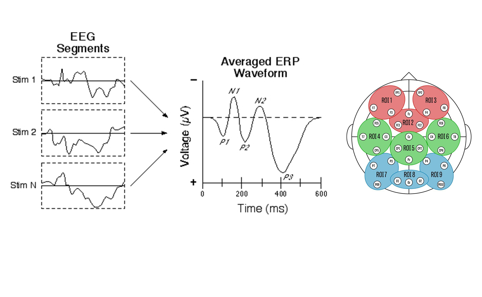
ERPs to study grammatical gender violations

A P600 (a positivity ‘around’ 600 ms. after stimulus onset) is sensitive to grammatical violations
An N400 (a negativity ‘around’ 400 ms. after stimulus onset) is modulated by semantic context and lexical properties of a word
- The P600/N400 are found by comparing incorrect to correct sentences
Native speakers appear to show a P600 for grammatical gender violations
- But analyzed by averaging over items and over subjects!

This study

In this study we are interested in how non-native speakers respond to grammatical gender violations (joint work with Nienke Meulman)
Grammatical gender is very hard to learn for L2 learners
Even though behaviorally L2 learners might show correct responses, the brain may reveal differences in processing grammatical gender

Research question

Is the P600 for grammatical gender violations dependent on age of arrival for the L2 learners of German?

ERP data

Today: analysis of single region of interest (ROI 8)

Design

67 L2 speakers of German (Slavic L1)
Auditory presentation of correct sentences or sentences with a grammatical gender violation (incorrect determiner; no determiners in L1)
48 items in each condition: 96 trials per participant (minus artifacts)
Example:

Nach der Schlägerei ist das / *der Auge des Angestellten von der Krankenschwester versorgt worden.

[After the fight theneut / *themasc eye of the worker was treated by the nurse]

Data overview

load('dat.rda')
dat = dat[order(dat$Subject, dat$TrialNr, dat$Time), ] # sort data per trial
dat$start.event <- dat$Time == min(dat$Time) # mark the start of every new trial 
head(dat)

       uV Time Subject Word TrialNr  Type AoArr start.event
721  8.94  505   GL102 Wald       2 incor     8        TRUE
722 15.56  515   GL102 Wald       2 incor     8       FALSE
723 21.31  525   GL102 Wald       2 incor     8       FALSE
724 13.32  535   GL102 Wald       2 incor     8       FALSE
725 19.11  545   GL102 Wald       2 incor     8       FALSE
726 17.96  555   GL102 Wald       2 incor     8       FALSE

dim(dat) # signal was downsampled to 100 Hz

[1] 442160      8

Much individual variation

General patterns exist

(note the arbitrary age splits, however)

Question 1

Investigating difference between correct and incorrect

(R version 4.4.2 (2024-10-31 ucrt), `mgcv` version 1.9.3, `itsadug` version 2.4.1)

library(mgcv)
library(itsadug)

# duration discrete=F: 3000s.; 1/2/4 threads: 230/120/65 s.
system.time(m0 <- bam(uV ~ s(Time,by=Type) + Type + s(Time,Subject,by=Type,bs='fs',m=1) +
                           s(Time,Word,by=Type,bs='fs',m=1), data=dat, rho=rhoval, 
                      AR.start=dat$start.event, discrete=T, nthreads=8))

   user  system elapsed 
 193.20    2.85   34.52

Time window was set to [500,1300] to limit CPU time
ACF of model without rho was used to determine rhoval: 0.91
Note that the difference between correct and incorrect will be overly conservative

Global difference between correct and incorrect

summary(m0) # slides only show the relevant part of the summary

Parametric coefficients:
            Estimate Std. Error t value Pr(>|t|) 
(Intercept)   -0.561      0.521   -1.08    0.282 
Typeincor      0.803      0.670    1.20    0.231 

Approximate significance of smooth terms:
                            edf Ref.df    F  p-value    
s(Time):Typecor            1.11   1.20 0.24    0.635    
s(Time):Typeincor          3.32   4.32 6.77 1.65e-05 ***
s(Time,Subject):Typecor   58.99 603.00 0.90   <2e-16 ***
s(Time,Subject):Typeincor 53.97 602.00 0.48   <2e-16 ***
s(Time,Word):Typecor      68.31 864.00 0.29   <2e-16 ***
s(Time,Word):Typeincor    65.86 863.00 0.26   <2e-16 ***

Deviance explained = 5.2%

Visualizing difference between correct and incorrect

plot_smooth(m0, view='Time', rug=F, plot_all='Type', main='') 
plot_diff(m0, view='Time', comp=list(Type=c('incor','cor'))) # overly conservative

Modeling the difference directly using a binary curve

dat$IsIncorrect <- (dat$Type == 'incor')*1 # create binary predictor: 0 = cor, 1 = incor
m0b <- bam(uV ~ s(Time) + s(Time,by=IsIncorrect) + s(Time,Subject,bs='fs',m=1) +
              s(Time,Subject,by=IsIncorrect,bs='fs',m=1) + s(Time,Word,bs='fs',m=1) +
              s(Time,Word,by=IsIncorrect,bs='fs',m=1), data=dat, rho=rhoval, 
           AR.start=dat$start.event, discrete=T, nthreads=8)

s(Time, by=IsIncorrect) is equal to 0 whenever IsIncorrect equals 0
Correct case: s(Time) + 0 = s(Time)
Incorrect case: s(Time) + s(Time, by=IsIncorrect)
- Difference between correct and incorrect: s(Time, by=IsIncorrect)
- Binary curve difference is non-centered (i.e. includes intercept difference)
This approach is not overly conservative, as the dependency between the nonlinear patterns for the correct and incorrect case per subject (and word) in the random effects is explicitly included (Sóskuthy, 2021)

Results using a binary curve

summary(m0b, re.test = FALSE) # summary without random effects (quicker to compute)

Parametric coefficients:
            Estimate Std. Error t value Pr(>|t|) 
(Intercept)   -0.573      0.468   -1.22    0.221 

Approximate significance of smooth terms:
                     edf Ref.df   F p-value    
s(Time)             1.64   2.05 0.6   0.535    
s(Time):IsIncorrect 4.08   5.00 3.9   0.002 **

s(Time):IsIncorrect shows the significance of the combined intercept and non-linear difference between correct and incorrect

Modeling the difference using an ordered factor

dat$TypeO <- as.ordered(dat$Type) # creating an ordered factor ...
contrasts(dat$TypeO) <- 'contr.treatment' # ... with contrast treatment: cor = 0, incor = 1
m0o <- bam(uV ~ s(Time) + s(Time,by=TypeO) + TypeO + s(Time,Subject,bs='fs',m=1) +
              s(Time,Subject,by=TypeO,bs='fs',m=1) + s(Time,Word,bs='fs',m=1) + 
              s(Time,Word,by=TypeO,bs='fs',m=1), data=dat, rho=rhoval, 
           AR.start=dat$start.event, discrete=T, nthreads=8)

s(Time, by=TypeO) is equal to 0 whenever TypeO equals cor (reference level)
Difference between correct and incorrect: s(Time, by=TypeO) + TypeO
- s(Time, by=TypeO): centered non-linear difference
- TypeO (must be included): intercept difference
The random-effects specification is effectively the same as that of the binary curve model, given that factor smooths involving ordered factors are not centered
This random reference/difference smooths approach (Sóskuthy, 2021) is appropriate and not overly conservative

Results using an ordered factor

summary(m0o, re.test = FALSE)

Parametric coefficients:
            Estimate Std. Error t value Pr(>|t|) 
(Intercept)   -0.573      0.468   -1.22    0.221 
TypeOincor     0.789      0.575    1.37    0.170 

Approximate significance of smooth terms:
                    edf Ref.df    F p-value    
s(Time)            1.64   2.05 0.60   0.535    
s(Time):TypeOincor 3.08   4.00 4.58   0.001 **

The \(p\)-value of the parametric coefficient TypeOincor represents the significance of the intercept difference between correct and incorrect
The \(p\)-value of the smooth term s(Time):TypeOincor represents the significance of the non-linear difference between correct and incorrect

Visualization of both difference curves

plot(m0b, select=2, scheme=1, rug=F, main='Binary difference', ylim=c(-3,3))
plot(m0o, select=2, scheme=1, rug=F, main='Ordered factor difference', ylim=c(-3,3))

Question 2

Testing our research question: a non-linear interaction

(`te` is used to model a non-linear interaction with predictors on a different scale)

m1 <- bam(uV ~ te(Time,AoArr,by=Type) + Type + s(Time,Subject,bs='fs',m=1) +
            s(Time,Subject,by=TypeO,bs='fs',m=1) + s(Time,Word,bs='fs',m=1) +
            s(Time,Word,by=TypeO,bs='fs',m=1), data=dat, rho=rhoval, 
          AR.start = dat$start.event, discrete=T, nthreads=8)
summary(m1, re.test = FALSE)

Parametric coefficients:
            Estimate Std. Error t value Pr(>|t|) 
(Intercept)   -0.457      0.472   -0.97    0.333 
Typeincor      0.476      0.561    0.85    0.396 

Approximate significance of smooth terms:
                          edf Ref.df    F  p-value    
te(Time,AoArr):Typecor   3.09   3.18 1.64    0.177    
te(Time,AoArr):Typeincor 5.88   6.96 4.59 4.14e-05 ***

Deviance explained = 5%

Visualization of the two-dimensional difference

Note the default maximum number of edf’s per 2D tensor product: 24 (5\(^2\) - 1)

plot_diff2(m1, view=c('Time','AoArr'), comp=list(Type=c("incor","cor")))
fadeRug(dat$Time, dat$AoArr) # hide points without data

Interpreting the two-dimensional difference

Interpreting two-dimensional interactions

Decomposition: the pure effect of age of arrival

m2 <- bam(uV ~ s(Time,by=Type) + s(AoArr,by=Type) + ti(Time,AoArr,by=Type) + Type +
            s(Time,Subject,bs='fs',m=1) + s(Time,Subject,by=TypeO,bs='fs',m=1) + 
            s(Time,Word,bs='fs',m=1) + s(Time,Word,by=TypeO,bs='fs',m=1), data=dat, rho=rhoval,
          AR.start=dat$start.event, discrete=T, nthreads=8) # te(x,y) = s(x) + s(y) + ti(x,y)
summary(m2, re.test=FALSE)

Parametric coefficients:
            Estimate Std. Error t value Pr(>|t|) 
(Intercept)   -0.450      0.472   -0.95    0.341 
Typeincor      0.472      0.561    0.84    0.400 

Approximate significance of smooth terms:
                          edf Ref.df    F  p-value    
s(Time):Typecor          1.02   1.04 0.04    0.878    
s(Time):Typeincor        3.31   4.30 6.56 2.32e-05 ***
s(AoArr):Typecor         1.01   1.01 2.37    0.124    
s(AoArr):Typeincor       1.00   1.00 1.85    0.173    
ti(Time,AoArr):Typecor   1.04   1.08 2.19    0.128    
ti(Time,AoArr):Typeincor 2.10   2.96 0.39    0.718

A simpler model without the non-linear interaction

m3 <- bam(uV ~ s(Time,by=Type) + s(AoArr,by=Type) + Type + s(Time,Subject,bs='fs',m=1) +
            s(Time,Subject,by=TypeO,bs='fs',m=1) + s(Time,Word,bs='fs',m=1) +
            s(Time,Word,by=TypeO,bs='fs',m=1), data=dat, rho=rhoval, 
          AR.start=dat$start.event, discrete=T, nthreads=8) # ti-terms dropped
summary(m3, re.test=FALSE)

Parametric coefficients:
            Estimate Std. Error t value Pr(>|t|) 
(Intercept)   -0.448      0.472   -0.95    0.342 
Typeincor      0.474      0.561    0.84    0.399 

Approximate significance of smooth terms:
                    edf Ref.df    F  p-value    
s(Time):Typecor    1.01   1.03 0.35    0.554    
s(Time):Typeincor  3.32   4.32 6.77 1.65e-05 ***
s(AoArr):Typecor   1.06   1.07 2.28    0.134    
s(AoArr):Typeincor 1.01   1.01 1.80    0.179

While both age of arrival smooths are non-significant, this does not mean that their difference (i.e. the P600) is also non-significant

Model comparison: workaround to use `fREML`

m2.alt <- bam(uV ~ s(Time,by=Type) + s(AoArr,by=Type) + ti(Time,AoArr,by=Type) + Type +
                s(Time,Subject,bs='fs',m=1) + s(Time,Subject,by=TypeO,bs='fs',m=1) +
                s(Time,Word,bs='fs',m=1) + s(Time,Word,by=TypeO,bs='fs',m=1), data=dat, 
              rho=rhoval, AR.start=dat$start.event, select=T, discrete=T, nthreads=8) 

m3.alt <- bam(uV ~ s(Time,by=Type) + s(AoArr,by=Type) + Type + s(Time,Subject,bs='fs',m=1) +
                s(Time,Subject,by=TypeO,bs='fs',m=1) + s(Time,Word,bs='fs',m=1) +
                s(Time,Word,by=TypeO,bs='fs',m=1), data=dat, rho=rhoval, 
              AR.start=dat$start.event, select=T, discrete=T, nthreads=8)

If we set select = T, all smooths are considered random effects, and model comparison can be done using models fit with fREML (default fitting method)
- Advantage: discrete = T usable, and fREML fitting is much faster than ML
- Disadvantage: it is an approximation, the results will be less precise

Model comparison: results

compareML(m2.alt, m3.alt)

m2.alt: uV ~ s(Time, by = Type) + s(AoArr, by = Type) + ti(Time, AoArr, 
    by = Type) + Type + s(Time, Subject, bs = "fs", m = 1) + 
    s(Time, Subject, by = TypeO, bs = "fs", m = 1) + s(Time, 
    Word, bs = "fs", m = 1) + s(Time, Word, by = TypeO, bs = "fs", 
    m = 1)

m3.alt: uV ~ s(Time, by = Type) + s(AoArr, by = Type) + Type + s(Time, 
    Subject, bs = "fs", m = 1) + s(Time, Subject, by = TypeO, 
    bs = "fs", m = 1) + s(Time, Word, bs = "fs", m = 1) + s(Time, 
    Word, by = TypeO, bs = "fs", m = 1)

Chi-square test of fREML scores
-----
   Model   Score Edf Difference    Df p.value Sig.
1 m3.alt 1492275  18                              
2 m2.alt 1492273  24      1.450 6.000   0.821     

AIC difference: 4.89, model m3.alt has lower AIC.

No support to include ti-terms (simpler model m3.alt is better)

Question 3

Ordered factor model: significant differences

m4 <- bam(uV ~ s(Time) + s(Time,by=TypeO) + s(AoArr) + s(AoArr,by=TypeO) + TypeO +
            s(Time,Subject,bs='fs',m=1) + s(Time,Subject,by=TypeO,bs='fs',m=1) + 
            s(Time,Word,bs='fs',m=1) + s(Time,Word,by=TypeO,bs='fs',m=1), data=dat, 
          rho=rhoval, AR.start=dat$start.event, discrete=T, nthreads=8)
summary(m4, re.test = FALSE)

Parametric coefficients:
            Estimate Std. Error t value Pr(>|t|) 
(Intercept)   -0.411      0.475   -0.87    0.387 
TypeOincor     0.435      0.564    0.77    0.441 

Approximate significance of smooth terms:
                     edf Ref.df    F p-value    
s(Time)             1.64   2.05 0.60   0.535    
s(Time):TypeOincor  3.08   4.00 4.58   0.001 ** 
s(AoArr)            1.04   1.04 2.33   0.131    
s(AoArr):TypeOincor 1.00   1.00 9.10   0.003 **

Difference curves

plot(m4, select=2, scheme=1, rug=F, ylim=c(-3,3))
plot(m4, select=4, scheme=1, rug=F, ylim=c(-6,6))

Finally: model criticism

library(car)
qqp(resid(m4)) # quantile-quantile plot function from library car
hist(resid(m4))

Problematic residuals!

This type of residual distribution is common for EEG data
These extreme deviations are problematic and may affect \(p\)-values
Distribution of residuals looks like scaled-\(t\) distribution
- We can fit this type of model in bam: family="scat"

Fitting a scaled-\(t\) model: slower!

system.time(
  m4.scat <- bam(uV ~ s(Time) + s(Time,by=TypeO) + s(AoArr) + s(AoArr,by=TypeO) + TypeO + 
                    s(Time,Subject,bs='fs',m=1) + s(Time,Subject,by=TypeO,bs='fs',m=1) + 
                    s(Time,Word,bs='fs',m=1) + s(Time,Word,by=TypeO,bs='fs',m=1), data=dat, 
                 family="scat", rho=rhoval, AR.start=dat$start.event, discrete=T, nthreads=8))

   user  system elapsed 
 4496.6    44.4   665.5

# For comparison, duration of the Gaussian model
system.time(
  m4 <- bam(uV ~ s(Time) + s(Time,by=TypeO) + s(AoArr) + s(AoArr,by=TypeO) + TypeO + 
               s(Time,Subject,bs='fs',m=1) + s(Time,Subject,by=TypeO,bs='fs',m=1) + 
               s(Time,Word,bs='fs',m=1) + s(Time,Word,by=TypeO,bs='fs',m=1), data=dat, 
             rho=rhoval, AR.start=dat$start.event, discrete=T, nthreads=8))

   user  system elapsed 
 192.05    4.51   35.18

Using the scaled-\(t\) distribution: \(p\)-values change

summary(m4, re.test = FALSE)$s.table # significance of smooths

                     edf Ref.df     F p-value
s(Time)             1.64   2.05 0.595 0.53482
s(Time):TypeOincor  3.08   4.00 4.581 0.00107
s(AoArr)            1.04   1.04 2.333 0.13057
s(AoArr):TypeOincor 1.00   1.00 9.099 0.00253

summary(m4.scat, re.test = FALSE)$s.table # significance of smooths

                     edf Ref.df     F p-value
s(Time)             2.35   3.03 1.259 0.28801
s(Time):TypeOincor  3.12   4.04 4.364 0.00153
s(AoArr)            1.10   1.11 0.501 0.54432
s(AoArr):TypeOincor 1.01   1.02 8.433 0.00364

Using the scaled-\(t\) distribution: similar patterns

Model criticism: much improved!

par(mfrow=c(1,2))
qqp(resid(m4), main='m4') 
qqp(resid(m4.scat), main='m4.scat')

Discussion and conclusion

GAMs are very useful to analyze EEG and other time-series data
- GAMs can detect non-linear patterns, while taking into account individual variation and autocorrelation
- Using the random reference/difference smooths approach results in appropriate (not overly conservative) difference smooths (Sóskuthy, 2021)
- The by-approach (e.g., model m0) is better for modeling individual factor levels
- Associated paper: Meulman et al. (2015) (paper package: data and code)
Still work to do:
- Assessing by-word variability in the (linear) effect of age of arrival
- Testing the significance of other possibly important variables (e.g., proficiency)
- But stay close to your hypothesis: much unexplained variation in EEG data!

Recap

We have applied GAMs to EEG data and learned how to:
- Model difference smooths directly using binary predictors and ordered factors
- Use te(Time,AoArr) to model a non-linear interaction
- Decompose te(Time,AoArr) using ti() and two s()’s
- Use a scaled-\(t\) distribution to improve residuals
While we have analyzed a single region of interest, GAMs allow for spatial distribution analyses
- E.g., via te(x, y, Time, d = c(2,1))
Associated lab session:
- https://www.let.rug.nl/wieling/Statistics/GAM-EEG/lab

Evaluation

Questions?

Thank you for your attention!

https://www.martijnwieling.nl

m.b.wieling@rug.nl

Generalized additive models for EEG data

This lecture

ERPs to study grammatical gender violations

This study

Research question

ERP data

Design

Data overview

Much individual variation

General patterns exist

(note the arbitrary age splits, however)

Question 1

Investigating difference between correct and incorrect

(R version 4.4.2 (2024-10-31 ucrt), mgcv version 1.9.3, itsadug version 2.4.1)

Global difference between correct and incorrect

Visualizing difference between correct and incorrect

Modeling the difference directly using a binary curve

Results using a binary curve

Modeling the difference using an ordered factor

Results using an ordered factor

Visualization of both difference curves

Question 2

Testing our research question: a non-linear interaction

(te is used to model a non-linear interaction with predictors on a different scale)

Visualization of the two-dimensional difference

Note the default maximum number of edf’s per 2D tensor product: 24 (5\(^2\) - 1)

Interpreting the two-dimensional difference

Interpreting two-dimensional interactions

Decomposition: the pure effect of age of arrival

A simpler model without the non-linear interaction

Model comparison: workaround to use fREML

Model comparison: results

Question 3

Ordered factor model: significant differences

Difference curves

Finally: model criticism

Problematic residuals!

Fitting a scaled-\(t\) model: slower!

Using the scaled-\(t\) distribution: \(p\)-values change

Using the scaled-\(t\) distribution: similar patterns

Model criticism: much improved!

Discussion and conclusion

Recap

Evaluation

Questions?

(R version 4.4.2 (2024-10-31 ucrt), `mgcv` version 1.9.3, `itsadug` version 2.4.1)

(`te` is used to model a non-linear interaction with predictors on a different scale)

Model comparison: workaround to use `fREML`