
Introduction to Generalized Additive Modeling using articulography data
Lecture 3 of advanced regression for linguists
Martijn Wieling
Computational Linguistics Research Group
This lecture
- Introduction
- Generalized additive modeling
- Articulography
- Using articulography to study L2 pronunciation differences
- Design
- Methods:
Rcode - Results
- Discussion
Generalized additive modeling (1)
- Generalized additive model (GAM): relaxing assumption of linear relation between dependent variable and predictor
- Relationship between individual predictors and (possibly transformed) dependent variable is estimated by a non-linear smooth function: \(g(y) = s(x_1) +s(x_2,x_3) + a_4x_4 + ...\)
- Multiple predictors can be combined in a (hyper)surface smooth (next lecture)

- Multiple predictors can be combined in a (hyper)surface smooth (next lecture)
Question 1
Generalized additive modeling (2)
- Advantage of GAM over manual specification of non-linearities: the optimal shape of the non-linearity is determined automatically
- Appropriate degree of smoothness is automatically determined on the basis of cross validation to prevent overfitting
- Fitting minimizes combined error and "wigglyness"
- Number of basis functions limits the maximum amount of non-linearity
First ten basis functions

Generalized additive modeling (3)
- Choosing a smoothing basis
- Single predictor or isotropic predictors: thin plate regression spline (this lecture)
- Efficient approximation of the optimal (thin plate) spline
- Combining non-isotropic predictors: tensor product spline (next lecture)
- Single predictor or isotropic predictors: thin plate regression spline (this lecture)
- Generalized Additive Mixed Modeling:
- Random effects can be treated as smooths as well (Wood, 2008)
R:gamandbam(packagemgcv)
- For more (mathematical) details, see Wood (2006)
Articulography
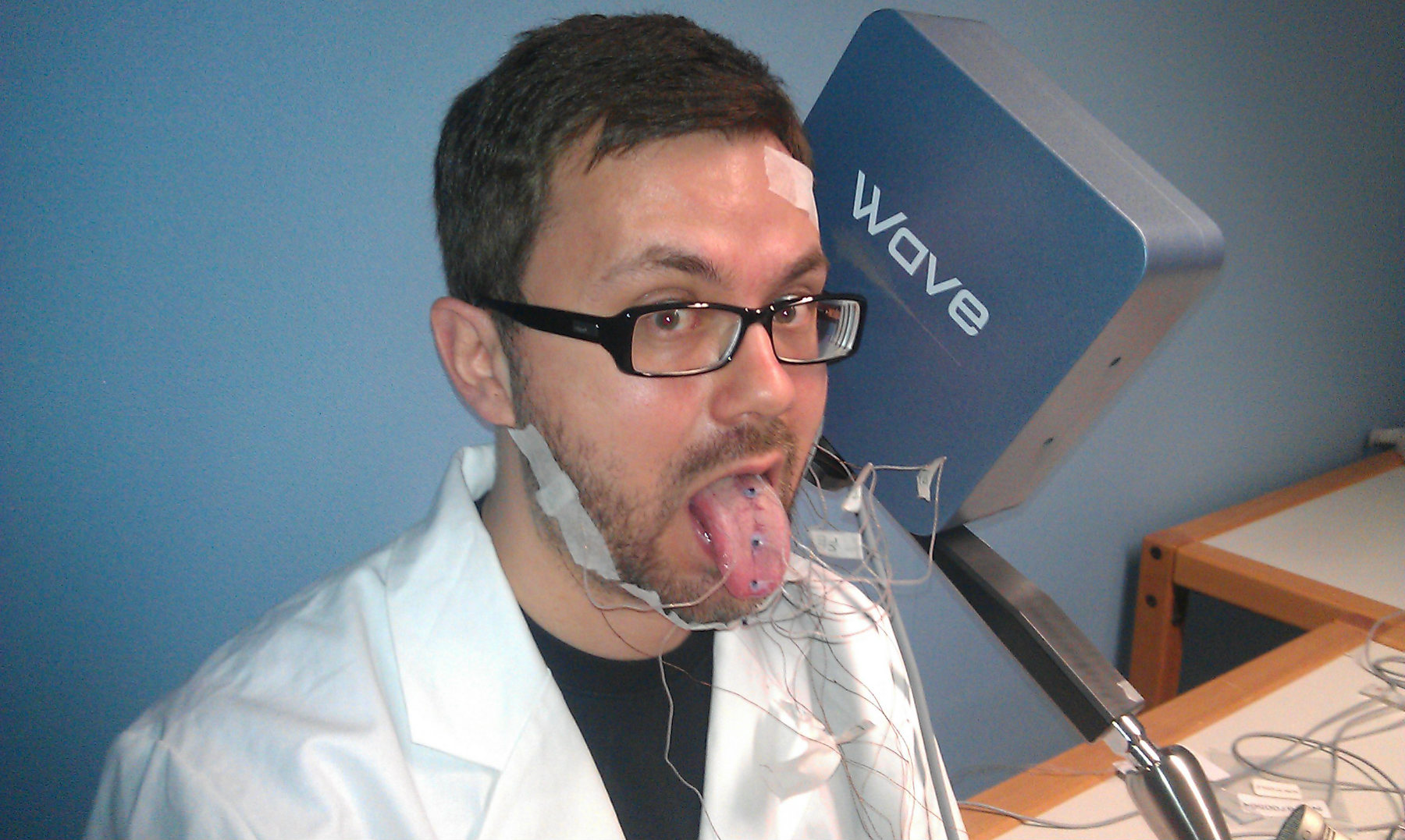
Obtaining data
Recorded data
Differences between native and non-native English
- 19 native Dutch speakers from Groningen
- 22 native Southern Standard British English speakers from London
- Material: 10 minimal pairs [t]:[θ] repeated twice:
- 'fate'-'faith', 'forth'-'fort', 'kit'-'kith', 'mitt'-'myth', 'tent'-'tenth'
- 'tank'-'thank', 'team'-'theme', 'tick'-'thick', 'ties'-'thighs', 'tongs'-'thongs'
- Note that the sound [θ] does not exist in the Dutch language
- The pronunciation of the words was preceded and followed by /ə/
- Goal: compare distinction between this sound contrast for both groups
- Preprocessing: Positions and time are normalized per speaker (between 0 and 1)
Data overview
load("art.rda")
head(art)
#          Word Axis Sensor Participant RecBlock    Time SeqNr Position Group Sound
# 112 @_faith_@    X     TB   VENI-EN_1        6 0.00278    21    0.842    EN    TH
# 113 @_faith_@    X     TB   VENI-EN_1        6 0.01065    21    0.844    EN    TH
# 114 @_faith_@    X     TB   VENI-EN_1        6 0.01852    21    0.843    EN    TH
# 115 @_faith_@    X     TB   VENI-EN_1        6 0.02639    21    0.842    EN    TH
# 116 @_faith_@    X     TB   VENI-EN_1        6 0.03426    21    0.842    EN    TH
# 117 @_faith_@    X     TB   VENI-EN_1        6 0.04213    21    0.839    EN    TH
dim(art)
# [1] 1083578 10
Much individual variation and noisy data

First model: tongue frontness for "theme" and "team"
(R version 3.3.2 (2016-10-31), mgcv version 1.8.16, itsadug version 2.2.4)
library(mgcv)
library(itsadug)
tm <- art[art$Word %in% c("@_theme_@", "@_team_@") & art$Sensor == "TT" & art$Axis == "X", ]
tm$TTfront <- 1 - tm$Position  # Position has higher values for backness: invert to represent frontness
tm <- start_event(tm, event = c("Participant", "Word", "RecBlock", "SeqNr"))  # sort data per individual trajectory
m0 <- bam(TTfront ~ s(Time), data = tm)
Model summary
summary(m0)
#
# Family: gaussian
# Link function: identity
#
# Formula:
# TTfront ~ s(Time)
#
# Parametric coefficients:
#             Estimate Std. Error t value Pr(>|t|)
# (Intercept) 0.766302   0.000621    1234   <2e-16 ***
# ---
# Signif. codes:  0 '***' 0.001 '**' 0.01 '*' 0.05 '.' 0.1 ' ' 1
#
# Approximate significance of smooth terms:
#          edf Ref.df   F p-value
# s(Time) 8.73   8.98 650  <2e-16 ***
# ---
# Signif. codes:  0 '***' 0.001 '**' 0.01 '*' 0.05 '.' 0.1 ' ' 1
#
# R-sq.(adj) =   0.24   Deviance explained = 24.1%
# fREML = -19420  Scale est. = 0.0071077  n = 18448
Visualizing the non-linear time pattern of the model
(Interpreting GAM results always involves visualization)
plot(m0, select = 1, rug = F, shade = T, main = "Partial effect", ylab = "TTfront")
plot_smooth(m0, view = "Time", rug = F, main = "Full effect")

Check if number of basis functions is adequate
(if p-value is low and edf close to k')
gam.check(m0)
#
# Method: fREML   Optimizer: perf newton
# full convergence after 10 iterations.
# Gradient range [-8.9e-06,8.16e-06]
# (score -19420 & scale 0.00711).
# Hessian positive definite, eigenvalue range [3.77,9223].
# Model rank =  10 / 10
#
# Basis dimension (k) checking results. Low p-value (k-index<1) may
# indicate that k is too low, especially if edf is close to k'.
#
#           k'  edf k-index p-value
# s(Time) 9.00 8.73    1.03    0.98
Increasing the number of basis functions with \(k\)
(double \(k\) if higher \(k\) is needed, but do not set it too high, i.e. max \(\frac{1}{2}\) \(\times\) unique time points)
m0b <- bam(TTfront ~ s(Time, k = 20), data = tm)
summary(m0b)$s.table  # new edf
#          edf Ref.df   F p-value
# s(Time) 13.2   15.7 373       0
summary(m0)$s.table # original edf
#          edf Ref.df   F p-value
# s(Time) 8.73   8.98 650       0
Effect of increasing \(k\)
plot_smooth(m0, view = "Time", rug = F, main = "m0 (k=10)")
plot_smooth(m0b, view = "Time", rug = F, main = "m0b (k=20)")

Including individual variation: random intercepts
(note the increased explained variance: was 24%)
m1 <- bam(TTfront ~ s(Time, k = 20) + s(Participant, bs = "re"), data = tm)
summary(m1)
#
# Family: gaussian
# Link function: identity
#
# Formula:
# TTfront ~ s(Time, k = 20) + s(Participant, bs = "re")
#
# Parametric coefficients:
#             Estimate Std. Error t value Pr(>|t|)
# (Intercept)  0.76911    0.00847    90.8   <2e-16 ***
# ---
# Signif. codes:  0 '***' 0.001 '**' 0.01 '*' 0.05 '.' 0.1 ' ' 1
#
# Approximate significance of smooth terms:
#                 edf Ref.df   F p-value
# s(Time)        14.4   16.8 587  <2e-16 ***
# s(Participant) 39.9   40.0 314  <2e-16 ***
# ---
# Signif. codes:  0 '***' 0.001 '**' 0.01 '*' 0.05 '.' 0.1 ' ' 1
#
# R-sq.(adj) =  0.548   Deviance explained =   55%
# fREML = -24100  Scale est. = 0.004224  n = 18448
Effect of including a random intercept
plot_smooth(m0b, view = "Time", rug = F, main = "m0b")
plot_smooth(m1, view = "Time", rug = F, main = "m1", rm.ranef = T)

Including individual variation: random slopes
m2 <- bam(TTfront ~ s(Time, k = 20) + s(Participant, bs = "re") + s(Participant, Time, bs = "re"), data = tm)
summary(m2)
#
# Family: gaussian
# Link function: identity
#
# Formula:
# TTfront ~ s(Time, k = 20) + s(Participant, bs = "re") + s(Participant,
#     Time, bs = "re")
#
# Parametric coefficients:
#             Estimate Std. Error t value Pr(>|t|)
# (Intercept)  0.76910    0.00948    81.1   <2e-16 ***
# ---
# Signif. codes:  0 '***' 0.001 '**' 0.01 '*' 0.05 '.' 0.1 ' ' 1
#
# Approximate significance of smooth terms:
#                      edf Ref.df     F p-value
# s(Time)             14.6   16.9   582  <2e-16 ***
# s(Participant)      39.4   40.0 44319  <2e-16 ***
# s(Participant,Time) 39.2   40.0 37380  <2e-16 ***
# ---
# Signif. codes:  0 '***' 0.001 '**' 0.01 '*' 0.05 '.' 0.1 ' ' 1
#
# R-sq.(adj) =   0.59   Deviance explained = 59.2%
# fREML = -24903  Scale est. = 0.0038396  n = 18448
Effect of including a random slope
plot_smooth(m1, view = "Time", rug = F, rm.ranef = T, main = "m1")
plot_smooth(m2, view = "Time", rug = F, rm.ranef = T, main = "m2")

Including individual variation: factor smooths
(i.e. including a non-linear random effect instead of a random intercept and random slope)
m3 <- bam(TTfront ~ s(Time, k = 20) + s(Time, Participant, bs = "fs", m = 1), data = tm)
summary(m3)
#
# Family: gaussian
# Link function: identity
#
# Formula:
# TTfront ~ s(Time, k = 20) + s(Time, Participant, bs = "fs", m = 1)
#
# Parametric coefficients:
#             Estimate Std. Error t value Pr(>|t|)
# (Intercept)   0.7687     0.0116    66.4   <2e-16 ***
# ---
# Signif. codes:  0 '***' 0.001 '**' 0.01 '*' 0.05 '.' 0.1 ' ' 1
#
# Approximate significance of smooth terms:
#                       edf Ref.df    F p-value
# s(Time)              14.4   16.6 22.9  <2e-16 ***
# s(Time,Participant) 318.5  368.0 68.2  <2e-16 ***
# ---
# Signif. codes:  0 '***' 0.001 '**' 0.01 '*' 0.05 '.' 0.1 ' ' 1
#
# R-sq.(adj) =  0.678   Deviance explained = 68.4%
# fREML = -26799  Scale est. = 0.0030093  n = 18448
Visualization of individual variation
plot(m3, select = 2)

Effect of including a random non-linear effect
plot_smooth(m2, view = "Time", rug = F, main = "m2", rm.ranef = T)
plot_smooth(m3, view = "Time", rug = F, main = "m3", rm.ranef = T)

Explore random effects yourself!
- Go to: http://eolomea.let.rug.nl/GAM/RandomEffects
- Login: p/s-number and RUG password, or:
f112300andShinyDem0
- Login: p/s-number and RUG password, or:
Speeding up computation
(via discrete and nthreads, only for default method="fREML")
system.time(bam(TTfront ~ s(Time, k = 20) + s(Time, Participant, bs = "fs", m = 1), data = tm))
#    user  system elapsed
#   7.568   0.311   7.885
system.time(bam(TTfront ~ s(Time, k = 20) + s(Time, Participant, bs = "fs", m = 1), data = tm, discrete = T))
#    user  system elapsed
#    2.70    0.08    2.79
system.time(bam(TTfront ~ s(Time, k = 20) + s(Time, Participant, bs = "fs", m = 1), data = tm, discrete = T,
    nthreads = 2))
#    user  system elapsed
#   3.141   0.105   2.627
- Note that the speed improvement when using
nthreadsis larger for more complex models
Comparing "theme" and "team" in one model
(smooths are centered, so the factorial predictor also needs to be included in the fixed effects)
m4 <- bam(TTfront ~ s(Time, by = Word, k = 20) + Word + s(Time, Participant, bs = "fs", m = 1), data = tm,
    discrete = T, nthreads = 2)
summary(m4)$p.table  # extract fixed effects from summary
#               Estimate Std. Error t value Pr(>|t|)
# (Intercept)     0.7480   0.011637    64.3        0
# Word@_theme_@   0.0416   0.000709    58.6        0
summary(m4)$s.table # extract non-linearities and random effects from summary
#                         edf Ref.df    F   p-value
# s(Time):Word@_team_@   13.3   15.6 16.1  6.24e-44
# s(Time):Word@_theme_@  14.5   16.7 36.2 4.02e-115
# s(Time,Participant)   327.6  368.0 89.9  0.00e+00
- Does the correct-incorrect distinction improve the model?
Assessing model improvement
(comparing fixed effects, so method='ML' and no discrete=T)
m3.ml <- bam(TTfront ~ s(Time, k = 20) + s(Time, Participant, bs = "fs", m = 1), data = tm, method = "ML")
m4.ml <- bam(TTfront ~ s(Time, by = Word, k = 20) + Word + s(Time, Participant, bs = "fs", m = 1), data = tm,
    method = "ML")
compareML(m3.ml, m4.ml)
# m3.ml: TTfront ~ s(Time, k = 20) + s(Time, Participant, bs = "fs", m = 1)
#
# m4.ml: TTfront ~ s(Time, by = Word, k = 20) + Word + s(Time, Participant,
#     bs = "fs", m = 1)
#
# Chi-square test of ML scores
# -----
#   Model  Score Edf    Chisq    Df  p.value Sig.
# 1 m3.ml -26805   5
# 2 m4.ml -29232   8 2426.205 3.000  < 2e-16  ***
#
# AIC difference: 4971.85, model m4.ml has lower AIC.
- Model
m4.mlis much better (AIC decrease > 2)!
Visualizing the two patterns
plot_smooth(m4, view = "Time", rug = F, plot_all = "Word", main = "m4", rm.ranef = T)

Visualizing the difference
plot_diff(m4, view = "Time", comp = list(Word = c("@_theme_@", "@_team_@")), ylim = c(-0.02, 0.12), rm.ranef = T)

Question 2
Including individual variation for "theme" vs. "team"
tm$ParticipantWord <- interaction(tm$Participant, tm$Word)  # new factor
m5 <- bam(TTfront ~ s(Time, by = Word, k = 20) + Word + s(Time, ParticipantWord, bs = "fs", m = 1), data = tm,
    discrete = T, nthreads = 2)
summary(m5)$p.table
#               Estimate Std. Error t value Pr(>|t|)
# (Intercept)     0.7486     0.0124   60.31   0.0000
# Word@_theme_@   0.0407     0.0176    2.32   0.0203
summary(m5)$s.table
#                           edf Ref.df    F  p-value
# s(Time):Word@_team_@     14.1   16.3 11.5 9.78e-31
# s(Time):Word@_theme_@    15.3   17.3 23.7 3.39e-75
# s(Time,ParticipantWord) 666.8  736.0 91.7 0.00e+00
More uncertainty in the difference
plot_diff(m4, view="Time", comp=list(Word=c("@_theme_@","@_team_@")), ylim=c(-0.05,0.15),
    main="m4: difference", rm.ranef=T)
plot_diff(m5, view="Time", comp=list(Word=c("@_theme_@","@_team_@")), ylim=c(-0.05,0.15),
    main="m5: difference", rm.ranef=T)

Autocorrelation in the data is a problem!
(residuals should be independent, otherwise the standard errors and p-values are wrong)
m5acf <- acf_resid(m5) # show autocorrelation

- Additional information: http://www.let.rug.nl/wieling/statscourse/ACF.pdf
Correcting for autocorrelation
(rhoval <- m5acf[2]) # correlation of residuals at time t with those at time t-1
#     1
# 0.956
m6 <- bam(TTfront ~ s(Time, by = Word, k = 20) + Word + s(Time, ParticipantWord, bs = "fs", m = 1), data = tm,
    rho = rhoval, AR.start = tm$start.event, discrete = T, nthreads = 2)
summary(m6)$p.table
#               Estimate Std. Error t value Pr(>|t|)
# (Intercept)     0.7485     0.0116   64.44   0.0000
# Word@_theme_@   0.0406     0.0164    2.47   0.0136
summary(m6)$s.table
#                           edf Ref.df     F  p-value
# s(Time):Word@_team_@     15.5   17.6 11.57 3.48e-33
# s(Time):Word@_theme_@    16.6   18.2 24.56 6.76e-82
# s(Time,ParticipantWord) 550.3  737.0  5.09 0.00e+00
Autocorrelation has been removed
par(mfrow = c(1, 2))
acf_resid(m5, main = "ACF of m5")
acf_resid(m6, main = "ACF of m6")

Clear model improvement
compareML(m5.ml, m6.ml)
# m5.ml: TTfront ~ s(Time, by = Word, k = 20) + Word + s(Time, ParticipantWord,
#     bs = "fs", m = 1)
#
# m6.ml: TTfront ~ s(Time, by = Word, k = 20) + Word + s(Time, ParticipantWord,
#     bs = "fs", m = 1)
#
# Model m6.ml preferred: lower ML score (24976.885), and equal df (0.000).
# -----
#   Model  Score Edf Difference    Df
# 1 m5.ml -33287   8
# 2 m6.ml -58264   8 -24976.885 0.000
#
# AIC difference: 48750.28, model m6.ml has lower AIC.
Explore autocorrelation yourself!
Question 3
Distinguishing the two speaker groups
tm$WordGroup <- interaction(tm$Word, tm$Group)
m7 <- bam(TTfront ~ s(Time, by = WordGroup, k = 20) + WordGroup + s(Time, ParticipantWord, bs = "fs",
    m = 1), data = tm, rho = rhoval, AR.start = tm$start.event, discrete = T, nthreads = 2)
summary(m7)$p.table
#                       Estimate Std. Error t value Pr(>|t|)
# (Intercept)             0.7257     0.0145   50.20 0.000000
# WordGroup@_theme_@.EN   0.0490     0.0205    2.40 0.016622
# WordGroup@_team_@.NL    0.0480     0.0212    2.26 0.023651
# WordGroup@_theme_@.NL   0.0792     0.0212    3.73 0.000196
summary(m7)$s.table
#                                 edf Ref.df     F  p-value
# s(Time):WordGroup@_team_@.EN   15.4   17.5 10.12 4.14e-28
# s(Time):WordGroup@_theme_@.EN  16.2   18.0 20.55 8.27e-67
# s(Time):WordGroup@_team_@.NL   10.1   12.8  3.84 3.66e-06
# s(Time):WordGroup@_theme_@.NL  13.6   16.2  7.83 4.91e-19
# s(Time,ParticipantWord)       530.6  735.0  4.43 0.00e+00
The difference between EN and NL is necessary
compareML(m6.ml, m7.ml)
# m6.ml: TTfront ~ s(Time, by = Word, k = 20) + Word + s(Time, ParticipantWord,
#     bs = "fs", m = 1)
#
# m7.ml: TTfront ~ s(Time, by = WordGroup, k = 20) + WordGroup + s(Time,
#     ParticipantWord, bs = "fs", m = 1)
#
# Chi-square test of ML scores
# -----
#   Model  Score Edf  Chisq    Df p.value Sig.
# 1 m6.ml -58264   8
# 2 m7.ml -58274  14 10.317 6.000   0.002  **
#
# AIC difference: 7.64, model m7.ml has lower AIC.
Visualizing the patterns
plot_smooth(m7, view = "Time", rug = F, plot_all = "WordGroup", main = "m7", rm.ranef = T)
plot_diff(m7, view = "Time", rm.ranef = T, ylim = c(-0.05, 0.2), comp = list(WordGroup = c("@_theme_@.EN",
    "@_team_@.EN")), main = "EN difference")
plot_diff(m7, view = "Time", rm.ranef = T, ylim = c(-0.05, 0.2), comp = list(WordGroup = c("@_theme_@.NL",
    "@_team_@.NL")), main = "NL difference")

The full tongue tip model: all words and both axes
(Word is now a random-effect factor, Sound distinguishes T from TH words)
t1 <- art[art$Sensor == "TT", ]
t1$GroupSoundAxis <- interaction(t1$Group, t1$Sound, t1$Axis)
t1$WordGroupAxis <- interaction(t1$Word, t1$Group, t1$Axis)
t1$PartSoundAxis <- interaction(t1$Participant, t1$Sound, t1$Axis)
t1 <- start_event(t1, event = c("Participant", "Word", "Axis", "RecBlock", "SeqNr"))

system.time(model <- bam(Position ~ s(Time, by = GroupSoundAxis, k = 20) + GroupSoundAxis + s(Time, PartSoundAxis,
    bs = "fs", m = 1) + s(Time, WordGroupAxis, bs = "fs", m = 1), data = t1, rho = rhoval, AR.start = t1$start.event,
    discrete = T, nthreads = 4))  # duration discrete=F: 1500 sec., discrete=T: 450 s. (1 thr.) / 260 s. (2 thr.)
#    user  system elapsed
#  537.81    4.55  155.86
The full tongue tip model: all words and both axes
smry <- summary(model)
smry$p.table
#                       Estimate Std. Error t value Pr(>|t|)
# (Intercept)            0.30975     0.0167 18.5301 1.28e-76
# GroupSoundAxisNL.T.X  -0.06384     0.0241 -2.6492 8.07e-03
# GroupSoundAxisEN.TH.X -0.05102     0.0245 -2.0851 3.71e-02
# GroupSoundAxisNL.TH.X -0.07036     0.0239 -2.9411 3.27e-03
# GroupSoundAxisEN.T.Z   0.06149     0.0251  2.4522 1.42e-02
# GroupSoundAxisNL.T.Z   0.07750     0.0257  3.0157 2.56e-03
# GroupSoundAxisEN.TH.Z  0.00137     0.0250  0.0547 9.56e-01
# GroupSoundAxisNL.TH.Z  0.03537     0.0255  1.3860 1.66e-01
smry$s.table
#                                   edf Ref.df     F   p-value
# s(Time):GroupSoundAxisEN.T.X    10.69   12.9  4.07  1.02e-06
# s(Time):GroupSoundAxisNL.T.X     9.88   12.2  3.20  1.11e-04
# s(Time):GroupSoundAxisEN.TH.X   14.33   15.6  5.58  4.93e-12
# s(Time):GroupSoundAxisNL.TH.X    9.17   11.5  1.69  6.85e-02
# s(Time):GroupSoundAxisEN.T.Z    18.46   18.6 55.54 3.88e-205
# s(Time):GroupSoundAxisNL.T.Z    18.06   18.3 30.65 9.70e-107
# s(Time):GroupSoundAxisEN.TH.Z   17.82   18.1 38.89 1.71e-137
# s(Time):GroupSoundAxisNL.TH.Z   16.68   17.3 13.06  3.91e-38
# s(Time,PartSoundAxis)         1353.95 1469.0 28.21  0.00e+00
# s(Time,WordGroupAxis)          629.79  713.0 46.93  0.00e+00
A clear L1-based pattern
plot_diff(model, view = "Time", rm.ranef = T, ylim = c(0.1, -0.15), comp = list(GroupSoundAxis = c("EN.TH.X",
    "EN.T.X")))
plot_diff(model, view = "Time", rm.ranef = T, ylim = c(0.1, -0.15), comp = list(GroupSoundAxis = c("NL.TH.X",
    "NL.T.X")))

2D visualization

Discussion
- Native English speakers appear to make the /t/-/θ/ distinction, whereas Dutch L2 speakers of English generally do not
- Obviously, the model could be improved by separating minimal pairs into two categories
Question 4
How to report?
- For an example of how to report this type of analysis, see:
- Wieling et al. (2016), Journal of Phonetics
- Data and
Rcode available online in Paper Package
Recap
- We have applied GAMs to articulography data and learned how to:
- use
s(Time)to model a non-linearity over time - use the
kparameter to control the number of basis functions - use the plotting functions
plot_smoothandplot_diff(rm.ranef=T!) - use the parameter setting
bs="re"to add random intercepts and slopes - add non-linear random effects using
s(Time,...,bs="fs",m=1) - use the
by-parameter to obtain separate non-linearities- Note that this factorial predictor needs to be included as fixed-effect factor as well!
- use
compareMLto compare models (method='ML'when comparing fixed effects)
- use
- After the break:
- Next lecture: more about generalized additive modeling using EEG data
Evaluation
Questions?
Thank you for your attention!