Analyzing EEG data using GAMs

Lecture 4 of advanced regression for linguists

Martijn Wieling
Computational Linguistics Research Group

This lecture

Introduction
- ERPs to study gender violations
- Research question
Design
Methods: R code
Results
Discussion

ERPs to study grammatical gender violations

A P600 (a positivity 'around' 600 ms. after stimulus onset) is sensitive to grammatical violations
An N400 (a negativity 'around' 400 ms. after stimulus onset) is modulated by semantic context and lexical properties of a word
- The P600/N400 are found by comparing the incorrect sentences to the correct sentences
Native speakers appear to show a P600 for gender violations
- But analyzed by averaging over items and over subjects!

This study

In this study we are interested in how non-native speakers respond to gender violations (joint work with Nienke Meulman)
Gender is very hard to learn for L2 learners
Even though behaviorally L2 learners might show correct responses, the brain may reveal differences in processing gender

Research question

Is the P600 for gender violations dependent on age of arrival for the L2 learners of German?

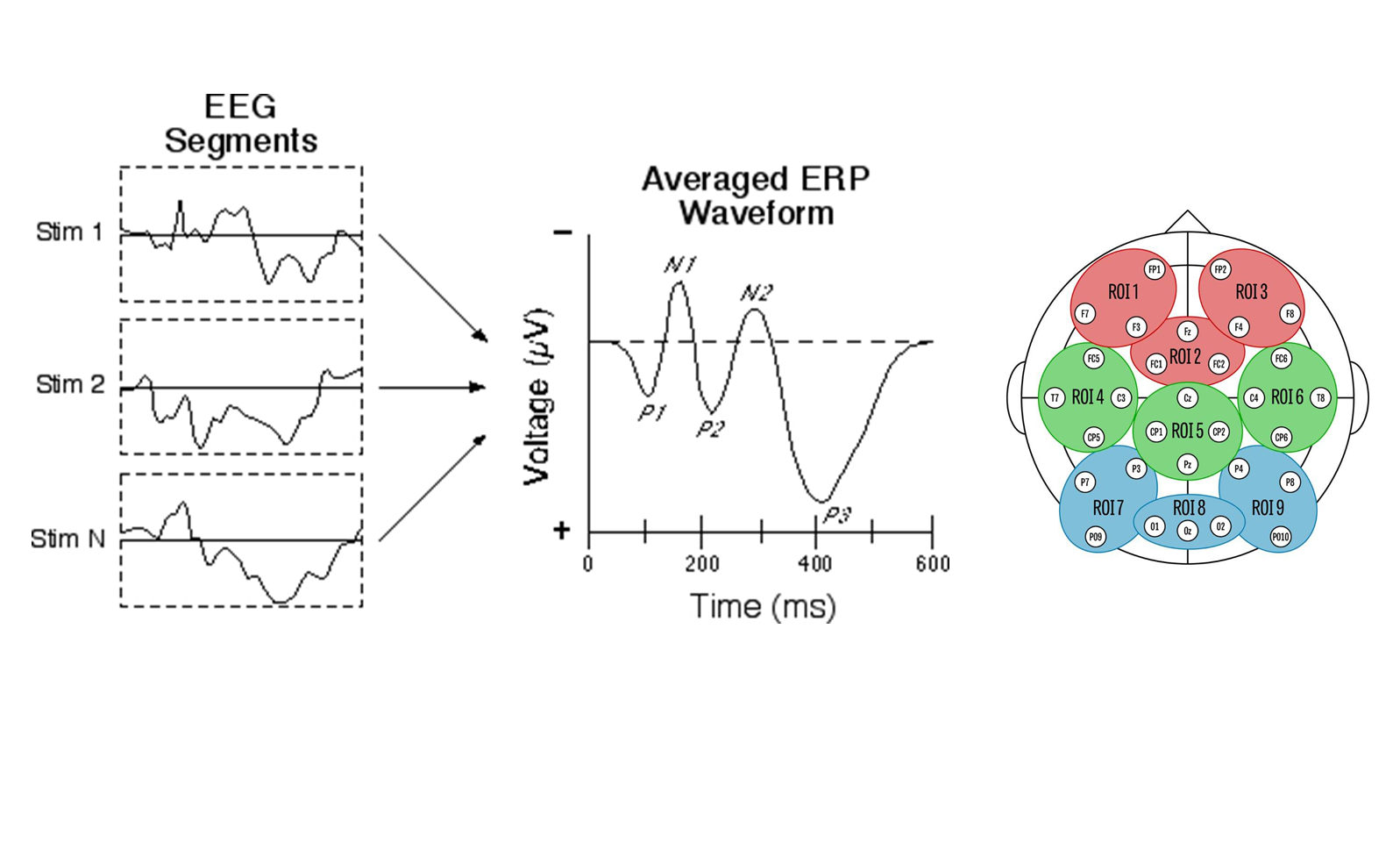
ERP data

Today: analysis of single region of interest (ROI 8)

Design

67 L2 speakers of German (Slavic L1)
Auditory presentation of correct sentences or sentences with a gender violation (incorrect determiner; no determiners in L1)
48 items in each condition: 96 trials per participant (minus artifacts)
Example:
Nach der Schlägerei ist das/*der Auge des Angestellten von der Krankenschwester versorgt worden.
After the fight theneut/*themasc eye of the worker was treated by the nurse

Data overview

(R version 3.3.2 (2016-10-31), `mgcv` version 1.8.16, `itsadug` version 2.2.4)

library(mgcv)
library(itsadug)
load("dat.rda")
dat <- start_event(dat, event = c("Subject", "TrialNr"))  # sorted data per subject and trial

head(dat)

#     uV Time Subject    Group Word TrialNr      Roi Structure Correctness L1 AoArr LoR Age Edu
# 1 37.6  505   GL103 GenEarly Brot       1 post.mid       DAN         cor RU     8  15  23   3
# 2 38.1  515   GL103 GenEarly Brot       1 post.mid       DAN         cor RU     8  15  23   3
# 3 39.9  525   GL103 GenEarly Brot       1 post.mid       DAN         cor RU     8  15  23   3
# 4 28.4  535   GL103 GenEarly Brot       1 post.mid       DAN         cor RU     8  15  23   3
# 5 34.8  545   GL103 GenEarly Brot       1 post.mid       DAN         cor RU     8  15  23   3
# 6 42.4  555   GL103 GenEarly Brot       1 post.mid       DAN         cor RU     8  15  23   3
#              AoAGroup start.event
# 1 Group 1: AoArr 7-12        TRUE
# 2 Group 1: AoArr 7-12       FALSE
# 3 Group 1: AoArr 7-12       FALSE
# 4 Group 1: AoArr 7-12       FALSE
# 5 Group 1: AoArr 7-12       FALSE
# 6 Group 1: AoArr 7-12       FALSE

dim(dat)

# [1] 442160     16

Much individual variation

(the signal has been downsampled to 100 Hz)

plot of chunk unnamed-chunk-2

General patterns exist

(note the arbitrary age splits, however)

plot of chunk unnamed-chunk-3

Question 1

Investigating difference between correct and incorrect

(for all participants; to limit CPU time, the time window was set to [500,1300])

dat$SubjectCor <- interaction(dat$Subject, dat$Correctness)
dat$WordCor <- interaction(dat$Word, dat$Correctness)
# duration discrete=F: 3000 sec.; 1/2/4/8/16 threads: 800/450/250/150/200 sec.
system.time(m0 <- bam(uV ~ s(Time, by = Correctness) + Correctness + s(Time, SubjectCor, bs = "fs", m = 1) + 
    s(Time, WordCor, bs = "fs", m = 1), data = dat, rho = rhoval, AR.start = dat$start.event, discrete = T, 
    nthreads = 2))

#    user  system elapsed 
# 869.004   0.044 450.301

system.time(smry0 <- summary(m0))  # storing summary as it also takes some time to compute

#    user  system elapsed 
#  75.777   0.004  75.830

Global difference between correct and incorrect

smry0  # show summary

# 
# Family: gaussian 
# Link function: identity 
# 
# Formula:
# uV ~ s(Time, by = Correctness) + Correctness + s(Time, SubjectCor, 
#     bs = "fs", m = 1) + s(Time, WordCor, bs = "fs", m = 1)
# 
# Parametric coefficients:
#                  Estimate Std. Error t value Pr(>|t|)
# (Intercept)        -0.553      0.473   -1.17     0.24
# Correctnessincor    0.733      0.670    1.09     0.27
# 
# Approximate significance of smooth terms:
#                             edf  Ref.df    F p-value    
# s(Time):Correctnesscor     1.04    1.08 0.39    0.57    
# s(Time):Correctnessincor   3.32    4.32 6.76 1.2e-05 ***
# s(Time,SubjectCor)       114.28 1204.00 0.69 < 2e-16 ***
# s(Time,WordCor)          134.33 1726.00 0.28 < 2e-16 ***
# ---
# Signif. codes:  0 '***' 0.001 '**' 0.01 '*' 0.05 '.' 0.1 ' ' 1
# 
# R-sq.(adj) =  0.0513   Deviance explained = 5.18%
# fREML = 1.4922e+06  Scale est. = 281.02    n = 442160

Visualizing difference between correct and incorrect

par(mfrow = c(1, 2))
plot_smooth(m0, view = "Time", rug = F, plot_all = "Correctness", main = "", rm.ranef = T, eegAxis = T)
plot_diff(m0, view = "Time", comp = list(Correctness = c("incor", "cor")), rm.ranef = T, eegAxis = T)

plot of chunk unnamed-chunk-6

Modeling the difference directly using a binary curve

dat$IsIncorrect <- (dat$Correctness == "incor") * 1  # creating a binary variable (incor: 1, cor: 0)
m0b <- bam(uV ~ s(Time) + s(Time, by = IsIncorrect) + s(Time, SubjectCor, bs = "fs", m = 1) + s(Time, 
    WordCor, bs = "fs", m = 1), data = dat, rho = rhoval, AR.start = dat$start.event, discrete = T, nthreads = 2)
# s(Time,by=IsIncorrect) = 0 when IsIncorrect = 0, otherwise it is a NON-CENTERED non-linear
# difference trajectory (i.e. including intercept difference)

smry0b <- summary(m0b)
smry0b$p.table

#             Estimate Std. Error t value Pr(>|t|)
# (Intercept)   -0.537      0.474   -1.13    0.257

smry0b$s.table  # p(s(Time):IsIncorrect): significance of the full cor-incor DIFFERENCE

#                        edf  Ref.df     F   p-value
# s(Time)               1.64    2.05 0.666  5.36e-01
# s(Time):IsIncorrect   4.08    5.00 3.833  1.80e-03
# s(Time,SubjectCor)  114.28 1204.00 0.688 1.46e-125
# s(Time,WordCor)     134.33 1726.00 0.275  7.19e-55

Modeling the difference using an ordered factor

dat$CorrectnessO <- as.ordered(dat$Correctness)  # creating an ordered factor ...
contrasts(dat$CorrectnessO) <- "contr.treatment"  # ... with contrast treatment
m0o <- bam(uV ~ s(Time) + s(Time, by = CorrectnessO) + CorrectnessO + s(Time, SubjectCor, bs = "fs", 
    m = 1) + s(Time, WordCor, bs = "fs", m = 1), data = dat, rho = rhoval, AR.start = dat$start.event, 
    discrete = T, nthreads = 2)
# s(Time,by=CorrecnessO) = 0 when CorrectnessO is at its reference level (cor), otherwise it is a
# CENTERED non-linear difference trajectory

smry0o <- summary(m0o)
smry0o$p.table  # p(CorrectnessOincor) indicates significance of the constant DIFFERENCE

#                   Estimate Std. Error t value Pr(>|t|)
# (Intercept)         -0.537      0.474   -1.13    0.257
# CorrectnessOincor    0.753      0.670    1.12    0.261

smry0o$s.table  # p(s(Time):CorrectnessOincor) indicates significance of non-linear DIFFERENCE

#                              edf  Ref.df     F   p-value
# s(Time)                     1.64    2.05 0.666  5.36e-01
# s(Time):CorrectnessOincor   3.08    4.00 4.578  1.08e-03
# s(Time,SubjectCor)        114.28 1204.00 0.688 1.47e-125
# s(Time,WordCor)           134.33 1726.00 0.275  7.19e-55

Visualization of both difference curves

par(mfrow = c(1, 2))
plot(m0b, select = 2, shade = T, rug = F, main = "Binary difference curve", ylim = c(3, -3))
plot(m0o, select = 2, shade = T, rug = F, main = "Ordered factor difference curve", ylim = c(3, -3))

plot of chunk unnamed-chunk-9

Question 2

Testing our research question: a non-linear interaction

(`te` is used to model a non-linear interaction with predictors on a different scale)

m1 <- bam(uV ~ te(Time, AoArr, by = Correctness) + Correctness + s(Time, SubjectCor, bs = "fs", m = 1) + 
    s(Time, WordCor, bs = "fs", m = 1), data = dat, rho = rhoval, AR.start = dat$start.event, discrete = T, 
    nthreads = 2)
smry1 <- summary(m1)
smry1$p.table

#                  Estimate Std. Error t value Pr(>|t|)
# (Intercept)        -0.489      0.469  -1.041    0.298
# Correctnessincor    0.595      0.665   0.895    0.371

smry1$s.table

#                                    edf  Ref.df     F   p-value
# te(Time,AoArr):Correctnesscor     3.10    3.19 1.680  1.52e-01
# te(Time,AoArr):Correctnessincor   5.88    6.95 4.912  1.60e-05
# s(Time,SubjectCor)              111.94 1202.00 0.659 2.24e-119
# s(Time,WordCor)                 134.38 1726.00 0.276  5.93e-55

Visualization of the 2-dimensional difference

Note the default maximum number of edf's per smooth: 24 (5\(^2\) - 1)

plot_diff2(m1, view = c("Time", "AoArr"), rm.ranef = T, comp = list(Correctness = c("incor", "cor")))
fadeRug(dat$Time, dat$AoArr)  # indicate points without data

plot of chunk unnamed-chunk-11

Interpreting the 2-dimensional interaction

(note that the \(y\)-axes are not inverted here)

plot of chunk unnamed-chunk-12

Interpret interactions yourself!

Go to: http://eolomea.let.rug.nl/GAM/InterpretingInteractions

Decomposition: the pure effect of age of arrival

m2 <- bam(uV ~ s(Time, by = Correctness) + s(AoArr, by = Correctness) + ti(Time, AoArr, by = Correctness) + 
    Correctness + s(Time, SubjectCor, bs = "fs", m = 1) + s(Time, WordCor, bs = "fs", m = 1), data = dat, 
    rho = rhoval, AR.start = dat$start.event, discrete = T, nthreads = 2)
smry2 <- summary(m2)
smry2$p.table

#                  Estimate Std. Error t value Pr(>|t|)
# (Intercept)        -0.478      0.470   -1.02    0.308
# Correctnessincor    0.579      0.665    0.87    0.384

smry2$s.table

#                                    edf  Ref.df     F   p-value
# s(Time):Correctnesscor            1.04    1.09 0.158  7.40e-01
# s(Time):Correctnessincor          3.32    4.31 6.756  1.27e-05
# s(AoArr):Correctnesscor           1.03    1.04 2.588  1.10e-01
# s(AoArr):Correctnessincor         1.05    1.05 3.714  4.76e-02
# ti(Time,AoArr):Correctnesscor     1.06    1.11 2.058  1.33e-01
# ti(Time,AoArr):Correctnessincor   1.93    2.64 0.336  7.08e-01
# s(Time,SubjectCor)              111.86 1202.00 0.654 7.14e-119
# s(Time,WordCor)                 134.38 1726.00 0.276  5.94e-55

A simpler model without the non-linear interaction

m3 <- bam(uV ~ s(Time, by = Correctness) + s(AoArr, by = Correctness) + Correctness + s(Time, SubjectCor, 
    bs = "fs", m = 1) + s(Time, WordCor, bs = "fs", m = 1), data = dat, rho = rhoval, AR.start = dat$start.event, 
    discrete = T, nthreads = 2)
smry3 <- summary(m3)
smry3$p.table

#                  Estimate Std. Error t value Pr(>|t|)
# (Intercept)        -0.475      0.470  -1.011    0.312
# Correctnessincor    0.582      0.666   0.873    0.383

smry3$s.table

#                              edf  Ref.df     F   p-value
# s(Time):Correctnesscor      1.01    1.03 0.375  5.54e-01
# s(Time):Correctnessincor    3.32    4.32 6.762  1.24e-05
# s(AoArr):Correctnesscor     1.05    1.06 2.705  1.04e-01
# s(AoArr):Correctnessincor   1.11    1.12 3.337  5.28e-02
# s(Time,SubjectCor)        111.78 1202.00 0.652 1.83e-118
# s(Time,WordCor)           134.38 1726.00 0.276  5.96e-55

Model comparison

(workaround to use `fREML` comparison with `discrete=T`; `select=T` treats smooths as random effects)

m2.alt <- bam(uV ~ s(Time, by = Correctness) + s(AoArr, by = Correctness) + ti(Time, AoArr, by = Correctness) + 
    Correctness + s(Time, SubjectCor, bs = "fs", m = 1) + s(Time, WordCor, bs = "fs", m = 1), data = dat, 
    rho = rhoval, AR.start = dat$start.event, method = "fREML", select = T, discrete = T, nthreads = 2)

m3.alt <- bam(uV ~ s(Time, by = Correctness) + s(AoArr, by = Correctness) + Correctness + s(Time, SubjectCor, 
    bs = "fs", m = 1) + s(Time, WordCor, bs = "fs", m = 1), data = dat, rho = rhoval, AR.start = dat$start.event, 
    method = "fREML", select = T, discrete = T, nthreads = 2)

compareML(m2.alt, m3.alt)

# m2.alt: uV ~ s(Time, by = Correctness) + s(AoArr, by = Correctness) + 
#     ti(Time, AoArr, by = Correctness) + Correctness + s(Time, 
#     SubjectCor, bs = "fs", m = 1) + s(Time, WordCor, bs = "fs", 
#     m = 1)
# 
# m3.alt: uV ~ s(Time, by = Correctness) + s(AoArr, by = Correctness) + 
#     Correctness + s(Time, SubjectCor, bs = "fs", m = 1) + s(Time, 
#     WordCor, bs = "fs", m = 1)
# 
# Chi-square test of fREML scores
# -----
#    Model   Score Edf Chisq    Df p.value Sig.
# 1 m3.alt 1492233  14                         
# 2 m2.alt 1492233  20 0.528 6.000   0.983     
# 
# AIC difference: 5.95, model m3.alt has lower AIC.

Question 3

Difference curves

par(mfrow = c(1, 2))
plot_diff(m3, view = "Time", comp = list(Correctness = c("incor", "cor")), rm.ranef = T, eegAxis = T)
plot_diff(m3, view = "AoArr", comp = list(Correctness = c("incor", "cor")), rm.ranef = T, eegAxis = T)

plot of chunk unnamed-chunk-16

Finally: model criticism

par(mfrow = c(1, 2))
qqp(resid_gam(m3))  # resid_gam takes autocorrelation into account
hist(resid_gam(m3))

plot of chunk unnamed-chunk-17

Problematic residuals!

This type of residual distribution is common for EEG data
These deviations are problematic and may affect \(p\)-values

Approach to normalize residuals

Model fitting using scaled-\(t\) distribution
- Implemented in gam: family="scat"
- Adding rho to gam possible via custom function (created by Natalya Pya)
- Unfortunately, gam is too slow, so a bam approach is in development
- Current state: implemented for fREML estimation with pre-specified scaled-\(t\) parameters (\(\theta\)) (see Meulman et al., 2015)
- Thus gam still necessary to determine (\(\theta\)) (but applied to subset / simpler model specification)

Estimating scaled-\(t\) parameters efficiently

Fit an intercept-only scaled-t gam model (including rho, method="REML") to all data and extract \(\theta\)
Fit the complete model without random effects as a scaled-\(t\) gam model (including rho, method="REML") to all data and extract \(\theta\)
Compare the models' \(\theta\) values:
- Small differences: use \(\theta\) of the complex model in the bam estimation
- Large differences: determine \(\theta\) by fittting the complete model specification (including random effects) to a small subset of the data (randomly select trials, compare \(\theta\) across a few runs)

Fitting a scaled-\(t\) model

source("bam.art.fit-v11.R")  # custom functions by Natalya Pya
g0 <- gam(uV ~ 1, data = dat, method = "REML", family = scat(rho = rhoval, AR.start = dat$start.event))  # takes 6 seconds
g1 <- gam(uV ~ s(Time, by = Correctness) + s(AoArr, by = Correctness) + Correctness, data = dat, method = "REML", 
    family = scat(rho = rhoval, AR.start = dat$start.event))  # takes 14 minutes
theta0 <- g0$family$getTheta(TRUE)
(theta1 <- g1$family$getTheta(TRUE))

# [1] 4.57 5.27

theta0 - theta1

# [1] 0.00275 0.00210

# the Gaussian model (m3) takes 250 sec. using 4 procs
system.time(m4.scat <- bam.art(uV ~ s(Time, by = Correctness) + s(AoArr, by = Correctness) + Correctness + 
    s(Time, SubjectCor, bs = "fs", m = 1) + s(Time, WordCor, bs = "fs", m = 1), data = dat, method = "fREML", 
    family = art(theta = theta1, rho = rhoval), AR.start = dat$start.event, discrete = T, nthreads = 4))

#     user   system  elapsed 
# 13213.34     7.68  3447.88

Using the scaled-\(t\) distribution: \(p\)-values change

summary(m3)$s.table

#                              edf  Ref.df     F   p-value
# s(Time):Correctnesscor      1.01    1.03 0.375  5.54e-01
# s(Time):Correctnessincor    3.32    4.32 6.762  1.24e-05
# s(AoArr):Correctnesscor     1.05    1.06 2.705  1.04e-01
# s(AoArr):Correctnessincor   1.11    1.12 3.337  5.28e-02
# s(Time,SubjectCor)        111.78 1202.00 0.652 1.83e-118
# s(Time,WordCor)           134.38 1726.00 0.276  5.96e-55

summary(m4.scat)$s.table

#                              edf  Ref.df      F   p-value
# s(Time):Correctnesscor      1.03    1.05  0.674  4.27e-01
# s(Time):Correctnessincor    4.17    5.38 14.267  1.40e-14
# s(AoArr):Correctnesscor     1.48    1.50  1.802  2.74e-01
# s(AoArr):Correctnessincor   1.00    1.00  6.915  8.55e-03
# s(Time,SubjectCor)        120.61 1204.00  1.453 1.25e-310
# s(Time,WordCor)           137.74 1727.00  0.301  4.44e-62

Using the scaled-\(t\) distribution: similar patterns

plot of chunk unnamed-chunk-19

Model criticism: much improved!

par(mfrow = c(1, 2))
qqp(resid_gam(m3), main = "m3")
qqp(resid(m4.scat), main = "m4.scat")  # resid of scat model takes autocorrelation into account

plot of chunk unnamed-chunk-20

Discussion

Still work to do:
- E.g., testing the significance of other possibly important variables (proficiency, age, etc.)
But don't make it too complex!
- There is much variation present in EEG data and adding very complex surfaces will almost certainly improve your model significantly
- Keep it simple, otherwise you won't be able to compute/interpret the results
- Also note that for hypothesis testing, it is essential not to conduct step-wise approaches

Conclusion

GAMs are very useful to analyze EEG and other time-series data
The method is very suitable to detect non-linear patterns, while taking into account individual variation and correcting for autocorrelation
The results of this study are published in PLOS ONE

Supplementary material, including code and results is available here

Recap

We have applied GAMs to EEG data and learned how to:
- model difference smooths directly using binary predictors and ordered factors
- use te(Time,AoArr) to model a non-linear interaction
- decompose te(Time,AoArr) using ti() and s()
- use a scaled-\(t\) distribution to improve residuals
  - (fitting this type of model for a complete data set may take a lot of CPU time, however)
While we have analyzed a single region of interest, GAMs allow for spatial distribution analyses
- E.g., via te(x, y, Time, d = c(2,1))
- See http://eolomea.let.rug.nl/GAM/ScalpEEG
After the break:
- http://www.let.rug.nl/wieling/statscourse/lecture4/lab
Next lecture: generalized additive logistic modeling using dialect data

Evaluation

Questions?

Thank you for your attention!

http://www.martijnwieling.nl
wieling@gmail.com