Statistiek I

Descriptive statistics

Martijn Wieling
University of Groningen

Question 1: last lecture

Last lecture

  • Why use statistics?
    • Summarize data (descriptive statistics)
    • Assess relationships in data (inferential statistics)
  • Introduction to RStudio and R
    • Variables and functions
    • Import, view and modify data in R
    • Some visualization and statistics in R

This lecture

  • Descriptive statistics vs. inferential statistics
  • Sample vs. population
  • (Types of) variables
  • Distribution of a variable
  • Measures of central tendency
  • Measures of variation
  • Standardized scores
  • Checking for a normal distribution

Descriptive vs. inferential statistics

  • Descriptive statistics:
    • Statistics used to describe (sample) data without further conclusions
      • Measures of central tendency: Mean, median, mode
      • Measures of variation (or spread): range, IQR, variance, standard deviation
  • Inferential statistics:
    • Investigate data of sample in order to infer patterns in the population
      • Statistical tests: \(t\)-test, \(\chi^2\)-test, etc.

Question 2

Sample vs. population

Why study a sample?

  • Studying the whole population is (almost always) practically impossible
  • Sample is a (selected) subset of population and thus more accessible
    • Selection of representative sample is very important!

Question 3

Variables and values

  • Statistics always involves variables
    • Relations: involve two variables (e.g., English grade vs. English score)
  • The values of the variables indicate properties of the cases (i.e. the individuals or entities you study)
Variable Example values
Sex male, female, …
English grade 4.6, 5.5, 6.3, 7.2, …
Year of birth 1990, 1991, 1993, …
Native language Dutch, German, English, …

Tabular representation of data

  • Each case is shown in a row
  • Each variable in a column
  • For part of our data:
participant year sex bl_edu study english_grade english_score
495 2023 F N OTHER 8 8.48
496 2023 M N IS 7 7.50
497 2023 F N OTHER 7 7.20
498 2023 F N LING 6 7.27
499 2023 M N IS 7 6.20
500 2023 M N IS 8 6.26

Types of variables: nominal and ordinal

  • Nominal (categorical) scale: unordered categories
    • Sex (frequently binary: two categories), Native language, etc.
  • Ordinal: ordered (ranked) scale, but amount of difference unclear
    • Rank of English profiency (in class), Likert scale (Rate on a scale from 1 to 5…)

Types of variables: numerical

  • Interval scale: numerical with meaningful difference but no true 0
    • Year of birth, temperature in Celsius
  • Ratio scale: numerical with meaningful difference and true 0
    • Number of questions correct, age
  • Scale of variable determines possible statistics
    • E.g., mean age is possible, but not mean native language

Question 4

Types of variables: summary

Question 5

Characterizing nom. variables: (relative) freq. table

table(dat$sex)  # absolute frequencies
# 
#   F   M 
# 346 154
prop.table(table(dat$sex))  # relative frequencies
# 
#     F     M 
# 0.692 0.308

Characterizing nominal variables: visualization

par(mfrow = c(1, 2))
barplot(table(dat$sex), col = c("pink", "lightblue"), main = "abs. frq.")
barplot(prop.table(table(dat$sex)), col = c("pink", "lightblue"), main = "rel. frq.")
plot of chunk unnamed-chunk-3

plot of chunk unnamed-chunk-3

Bad practice: pie charts

pie(table(dat$study), col = c("red", "cyan", "blue", "yellow"))
plot of chunk unnamed-chunk-4

plot of chunk unnamed-chunk-4

Question 6

Characterizing numerical variables: distribution

  • We are generally not interested in individual values of a variable, but rather all values and their frequency
  • This is captured by a distribution
    • Famous distribution: Normal distribution (“bell-shaped” curve): e.g., IQ scores
plot of chunk unnamed-chunk-5

plot of chunk unnamed-chunk-5

Distribution

  • Distribution of a variable shows variability of variable (i.e. frequency of values)
table(dat$english_grade)
# 
#   5 5.5   6 6.5   7 7.5   8 8.5   9 9.5 
#   6   2  76  12 191  21 148  15  26   3

Visualizing a distribution: histogram

  • Histogram shows frequency of all values in groups: \((a,b]\)
    • Look for general pattern, symmetry, outliers
hist(dat$english_grade, xlab = "English grade", main = "")
plot of chunk unnamed-chunk-8

plot of chunk unnamed-chunk-8

Visualizing a distribution: density curve

  • Density curve shows area proportional to the relative frequency
plot(density(dat$english_grade), main = "", xlab = "English grade")
plot of chunk unnamed-chunk-10

plot of chunk unnamed-chunk-10

Interpreting a density curve

plot of chunk unnamed-chunk-11

plot of chunk unnamed-chunk-11

  • The total area under a density curve is equal to 1
  • A density curve does not provide information about the frequency of one value
    • E.g., there might be no one who has scored a grade of exactly 6.1
  • It only provides information about an interval
    • E.g., more than 50% of the grades lie between 5.5 and 7.5

Interpreting a density curve: normal distribution

plot of chunk unnamed-chunk-12

plot of chunk unnamed-chunk-12

  • The normal distribution has convenient characteristics
    • Completely symmetric
    • Red area: (about) 68%
    • Red and green area: (about) 95%

Characterizing the distribution of numerical variables

  • A distribution can also be characterized by measures of center and variation
    • (skewness measures the symmetry of the distribution; not covered in this course)

Characterizing numerical variables: central tendency

  • Mode: most frequent element (for nominal data: only meaningful measure)
  • Median: when data is sorted from small to large, it is the middle value
  • Mean: arithmetical average

$$\bar{x} = \frac{x_1 + x_2 + \cdots + x_n}{n} = \frac{1}{n}\sum\limits_{i=1}^n x_i$$

  • (You need to be able to calculate the mean of a series of values by hand, so it is useful to remember the formula)

Question 7

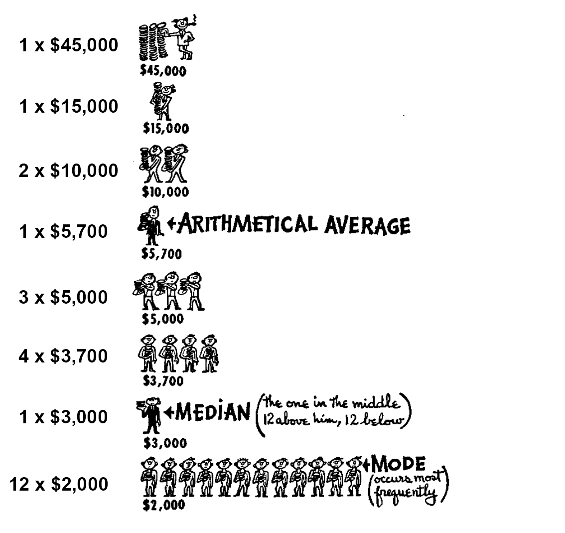
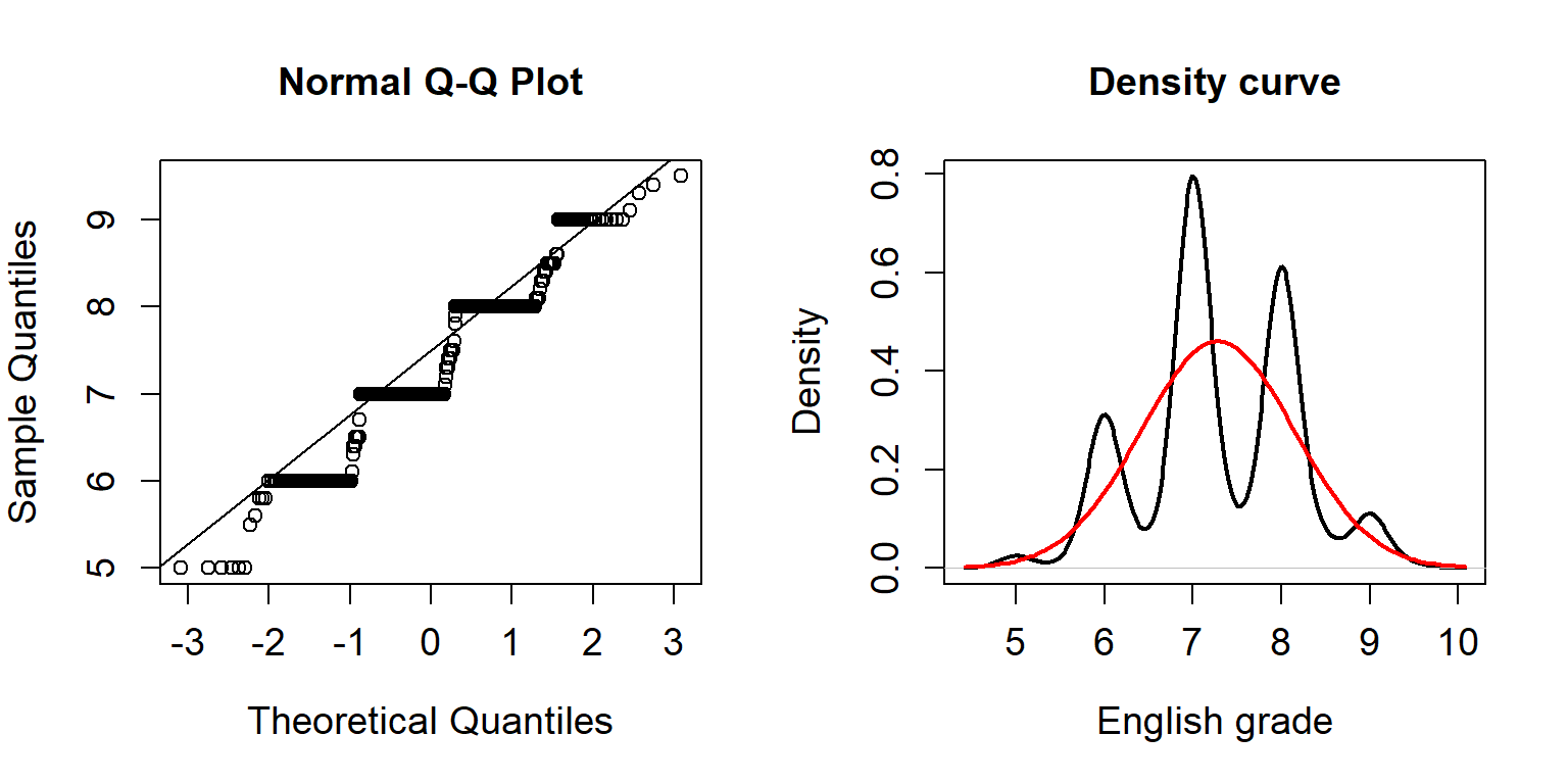
Measures of center may have very different values

Central tendency in R

mean(dat$english_grade)  # arithmetic average
# [1] 7.2828
median(dat$english_grade)
# [1] 7
# no built-in function to get mode: new function
my_mode <- function(x) {
    counts <- table(x)
    as.numeric(names(which(counts == max(counts))))
}
my_mode(dat$english_grade)
# [1] 7

Measure of variation: quantiles

  • Quantiles: cutpoints to divide the sorted data in subsets of equal size
    • Quartiles: three cutpoints to divide the data in four equal-sized sets
      • \(q_1\) (1st quartile): cutpoint between 1st and 2nd group
      • \(q_2\) (2nd quartile): cutpoint between 2nd and 3rd group (= median!)
      • \(q_3\) (3rd quartile): cutpoint between 3rd and 4th group
    • Percentiles: divide data in hundred equal-sized subsets
      • \(q_1\) = 25th percentile
      • \(q_2\) (= median) = 50th percentile
      • Score at \(n\)th percentile is better than \(n\)% of scores
quantile(dat$english_grade)  # default: quartiles
#   0%  25%  50%  75% 100% 
#  5.0  7.0  7.0  8.0  9.5

Measure of variation: range

  • Minimum, maximum: lowest and highest value
  • Range: difference between minimum and maximum
  • Interquartile range (IQR): \(q_3\) - \(q_1\)

Visualizing variation: box plot (box-and-whisker plot)

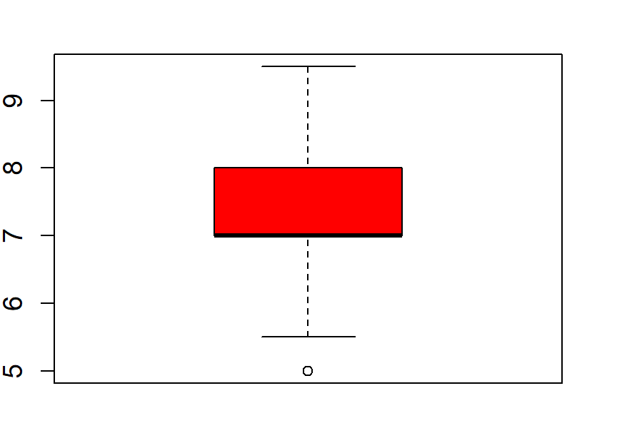
  • A box plot is used to visualize variation of a variable
    • Box (IQR): \(q_1\) (bottom), median (thickest line), \(q_3\) (top)
      • (In example below, \(q_1\) and median have the same value)
    • Whiskers: maximum (top) and minimum (bottom) non-outlier value
    • Circle(s): outliers (> 1.5 IQR distance from box)
boxplot(dat$english_grade, col = "red")
plot of chunk unnamed-chunk-16

plot of chunk unnamed-chunk-16

Important measure of variation: variance

  • Deviation: difference between mean and individual value
  • Variance: average squared deviation
    • Squared in order to make negative differences positive
    • Population variance (with \(\mu\) = population mean): $$\sigma^2 = \frac{1}{n}\sum\limits_{i=1}^n (x_i - \mu)^2$$
    • As sample mean ($\bar{x}$) is approximation of population mean ($\mu$), sample variance formula contains division by \(n-1\) (results in slightly higher variance): $$s^2 = \frac{1}{n-1}\sum\limits_{i=1}^n (x_i - \bar{x})^2$$

Important measure of variation: standard deviation

  • Standard deviation is square root of variance $$\sigma = \sqrt{\sigma^2} = \sqrt{\frac{1}{n}\sum\limits_{i=1}^n (x_i - \mu)^2}$$ $$s = \sqrt{s^2} = \sqrt{\frac{1}{n-1}\sum\limits_{i=1}^n (x_i - \bar{x})^2}$$

Question 8

Measures of variation (or spread) in R (1)

min(dat$english_grade)  # minimum value
# [1] 5
max(dat$english_grade)  # maximum value
# [1] 9.5
range(dat$english_grade)  # returns minimum and maximum value
# [1] 5.0 9.5
diff(range(dat$english_grade))  # returns difference between min. and max.
# [1] 4.5

Measures of variation (or spread) in R (2)

IQR(dat$english_grade)  # interquartile range
# [1] 1
var(dat$english_grade)  # sample variance
# [1] 0.75173
sd(dat$english_grade)  # sample standard deviation
# [1] 0.86702
sd(dat$english_grade) == sqrt(var(dat$english_grade))  # std. dev. = sqrt of var.?
# [1] TRUE

Normal distribution and standard deviation (1)

plot of chunk unnamed-chunk-19

plot of chunk unnamed-chunk-19

 
\(P(\mu - \sigma \leq x \leq \mu + \sigma) \approx 68\%\)     (34 + 34)
\(P(\mu - 2\sigma \leq x \leq \mu + 2\sigma) \approx 95\%\)     (34 + 34 + 13.5 + 13.5)
\(P(\mu - 3\sigma \leq x \leq \mu + 3\sigma) \approx 99.7\%\)     (34 + 34 + 13.5 + 13.5 + 2.35 + 2.35)

  • It is important to remember these characteristics of the normal distribution!

Normal distribution and standard deviation (2)

plot of chunk unnamed-chunk-20

plot of chunk unnamed-chunk-20

 
\(P(85 \leq \rm{IQ} \leq 115) \approx 68\%\)     (34 + 34)
\(P(70 \leq \rm{IQ} \leq 130) \approx 95\%\)     (34 + 34 + 13.5 + 13.5)
\(P(55 \leq \rm{IQ} \leq 145) \approx 99.7\%\)     (34 + 34 + 13.5 + 13.5 + 2.35 + 2.35)

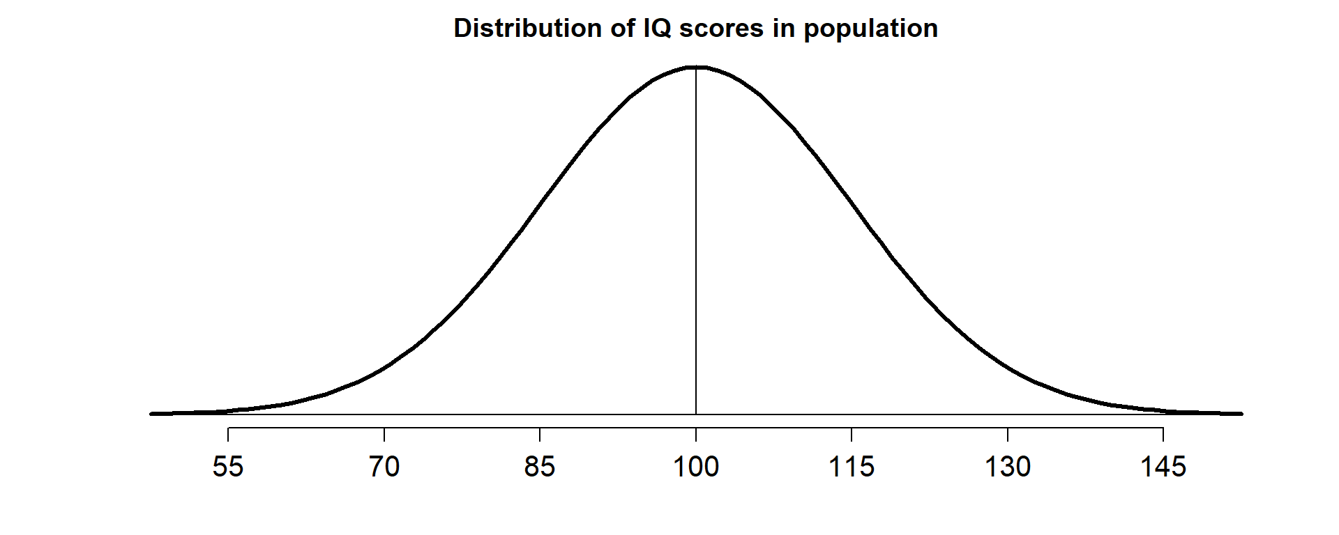
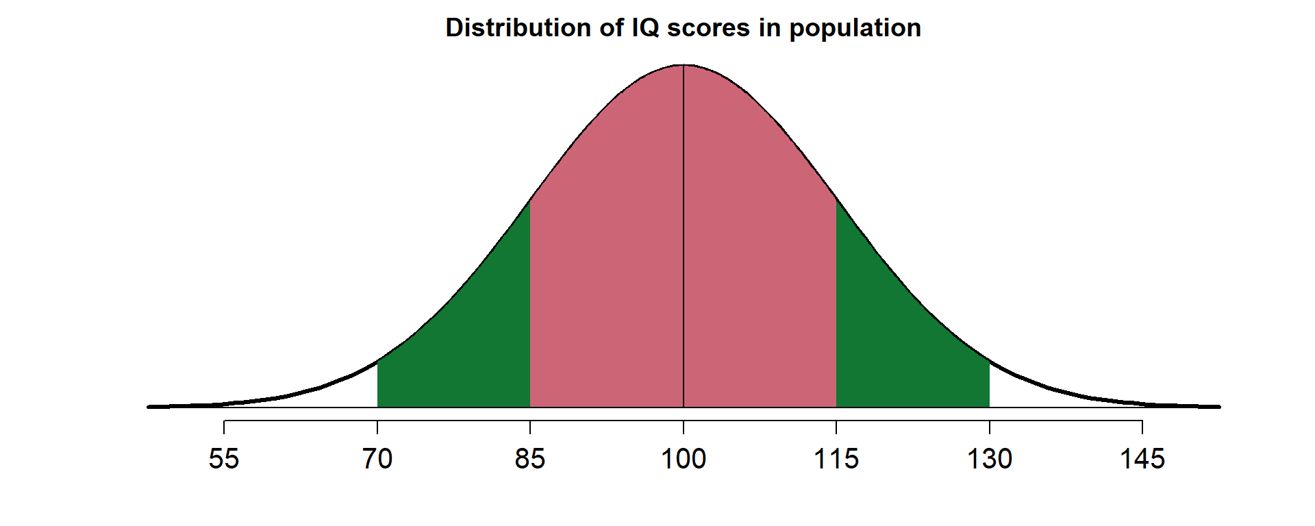
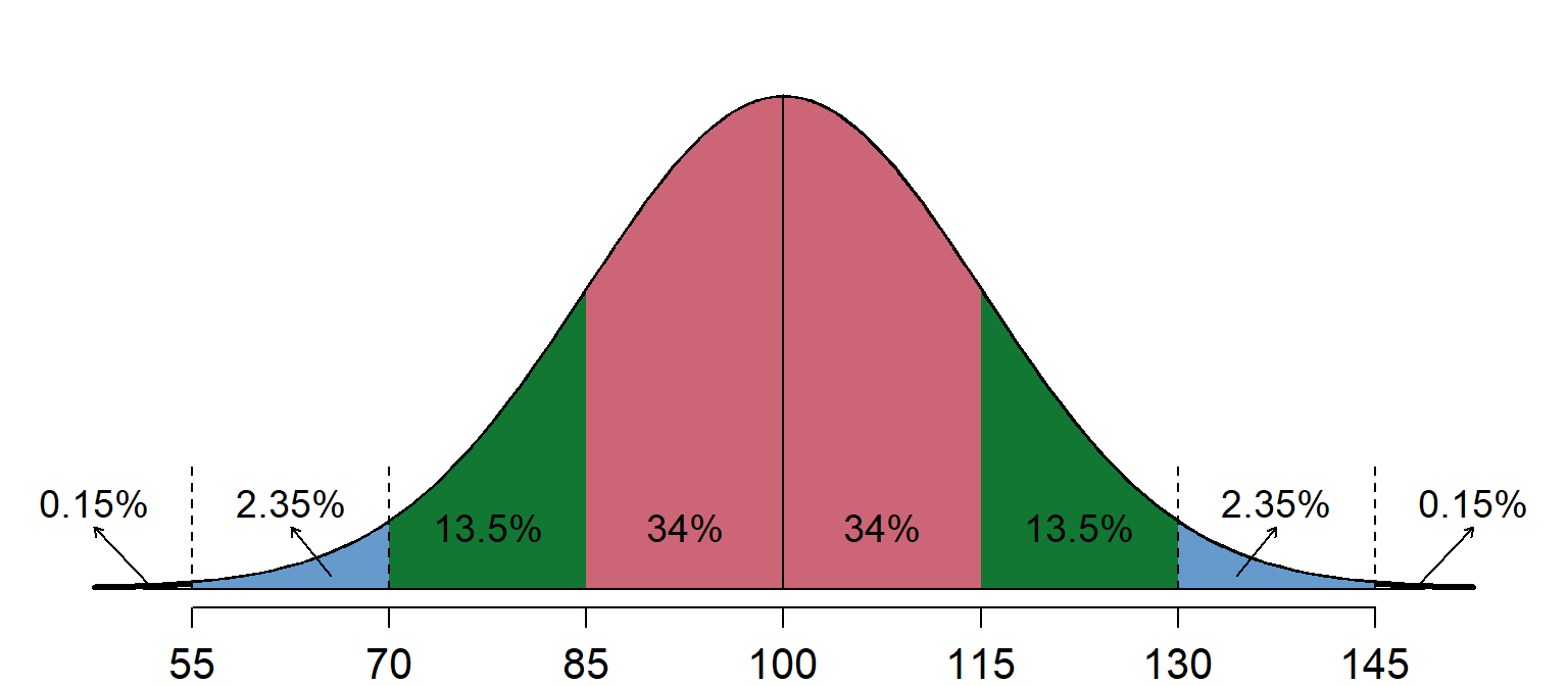
  • IQ scores are normally distributed with mean 100 and standard deviation 15

Standardized scores

  • Standardization helps facilitate interpretation
  • E.g., how to interpret: “Emma’s score is 112” and “David’s score is 105”
  • Interpretation should be done with respect to mean \(\mu\) and standard deviation \(\sigma\)
    • Raw scores can be transformed to standardized scores ($z$-scores or $z$-values) $$z = \frac{x - \mu}{\sigma} = \frac{\rm{deviation}}{\rm{standard}\,\rm{deviation}}$$
    • Interpretation: difference of value from mean in number of standard deviations
  • (Note that you have to be able to calculate \(z\)-scores!)

Calculating standardized values

  • Suppose \(\mu = 108\), \(\sigma = 4\), then: $$z_{112} = \frac{x - \mu}{\sigma} = \frac{112 - 108}{4} = 1$$ $$z_{105} = \frac{105 - 108}{4} = -0.75$$
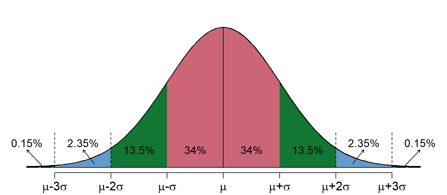
  • \(z\) shows distance from mean in number of standard deviations

Question 9

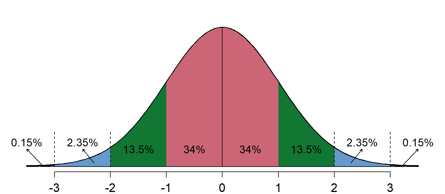
Distribution of standardized variables

  • If we transform all raw scores of a variable into \(z\)-scores using: $$z = \frac{x - \mu}{\sigma} = \frac{\rm{deviation}}{\rm{standard}\,\rm{deviation}}$$
  • We obtain a new transformed variable whose
    • Mean is 0
    • Standard deviation is 1
  • In sum: \(z\)-score = distance from \(\mu\) in \(\sigma\)’s
  • \(z\)-scores are useful for interpretation and hypothesis testing (next lecture)

Standardizing a variable in R

dat$english_grade.z <- scale(dat$english_grade)  # scale: calculates z-scores
mean(dat$english_grade.z)  # should be 0
# [1] 0
sd(dat$english_grade.z)  # should be 1
# [1] 1

Standard normal distribution

plot of chunk unnamed-chunk-23

plot of chunk unnamed-chunk-23

 
\(P(-1 \leq z \leq 1) \approx 68\%\)     (34 + 34)
\(P(-2 \leq z \leq 2) \approx 95\%\)     (34 + 34 + 13.5 + 13.5)
\(P(-3 \leq z \leq 3) \approx 99.7\%\)     (34 + 34 + 13.5 + 13.5 + 2.35 + 2.35)

For comparison: normal distribution

plot of chunk unnamed-chunk-24

plot of chunk unnamed-chunk-24

 
\(P(\mu - \sigma \leq x \leq \mu + \sigma) \approx 68\%\)     (34 + 34)
\(P(\mu - 2\sigma \leq x \leq \mu + 2\sigma) \approx 95\%\)     (34 + 34 + 13.5 + 13.5)
\(P(\mu - 3\sigma \leq x \leq \mu + 3\sigma) \approx 99.7\%\)     (34 + 34 + 13.5 + 13.5 + 2.35 + 2.35)

Percentiles and \(z\)-scores

  • If distribution is normal then \(z\)-scores correspond to percentiles
  • The function qnorm returns the \(z\)-values for a certain proportion (percentile / 100)
qnorm(95/100)  # z-value associated with 95th percentile
# [1] 1.6449
plot of chunk unnamed-chunk-25

plot of chunk unnamed-chunk-25

Question 10

\(z\)-scores and percentiles

  • The function pnorm returns the proportion of data < a specified \(z\)-value
    • the percentile can be found by multiplying with 100
100 * pnorm(1.6449)
# [1] 95
plot of chunk unnamed-chunk-26

plot of chunk unnamed-chunk-26

Some calculations with \(z\)-scores

  • What proportion of values have a \(z\)-value of at least 1.64?
    • \(P(z \geq 1.64)\)
1 - pnorm(1.64)
# [1] 0.050503
  • What proportion of values are located between \(z\)-values between -2 and 2?
    • \(P(-2 \leq z < 2)\)
pnorm(2) - pnorm(-2)
# [1] 0.9545

Visualization

pnorm(2)
# [1] 0.97725
pnorm(-2)
# [1] 0.02275
plot of chunk unnamed-chunk-29

plot of chunk unnamed-chunk-29

Question 11

Checking normality assumption

  • Some statistical tests require that the data is (roughly) normally distributed
  • How to test this?
    • Using visual inspection of a normal quantile plot (or: quantile-quantile plot)
      • A straight line in this graph indicates a (roughly) normal distribution
    • Using the Shapiro-Wilk test (covered in lecture 5)

Normal quantile plot: how it works

  • Sort the data from smallest to largest to determine quantiles (e.g., percentiles)
    • E.g., median for 50th percentile
  • Calculate \(z\)-values belonging to the quantiles (e.g., percentiles) of a standard normal distribution
    • E.g., \(z =\) 0 for 50th percentile, \(z =\) 2 for 97.5th percentile, etc.
  • Plot data values ($y$-axis) against normal quantile values ($x$-axis)
    • If points on (or close to) straight line: values normally distributed
  • (Note: you need to be able to interpret a quantile-quantile plot, but you don’t have to be able to construct the plot manually)

Normal quantile plot in R: English grades

qqnorm(dat$english_grade)
qqline(dat$english_grade)
plot of chunk unnamed-chunk-31

plot of chunk unnamed-chunk-31

  • Distribution not normal for the English grades

Normal quantile plot in R: English scores

qqnorm(dat$english_score)
qqline(dat$english_score)
plot of chunk unnamed-chunk-33

plot of chunk unnamed-chunk-33

  • Distribution roughly normal for the English scores

Recap

  • In this lecture, we’ve covered
    • Descriptive statistics vs. inferential statistics
    • Sample vs. population
    • Four types of variables
    • Distribution of a variable
    • Measures of central tendency
    • Measures of variation
    • Standardized scores
    • How to check for a normal distribution
  • In the lab session, you will experiment with descriptive statistics
  • Next lecture: Sampling

Please evaluate this lecture!

Exam question

Questions?

Thank you for your attention!

https://www.martijnwieling.nl
m.b.wieling@rug.nl