
Mixed-effects regression and eye-tracking data
Lecture 2 of advanced regression for linguists
Martijn Wieling
Computational Linguistics Research Group
This lecture
- Introduction
- Gender processing in Dutch
- Eye-tracking to reveal gender processing
- Design
- Analysis
- Conclusion
Gender processing in Dutch
- Study's goal: assess if Dutch people use grammatical gender to anticipate upcoming words
- This study was conducted together with Hanneke Loerts and is published in the Journal of Psycholinguistic Research (Loerts, Wieling and Schmid, 2012)
- What is grammatical gender?
- Gender is a property of a noun
- Nouns are divided into classes: masculine, feminine, neuter, ...
- E.g., hond ('dog') = common, paard ('horse') = neuter
- The gender of a noun can be determined from the forms of elements syntactically related to it
Gender in Dutch
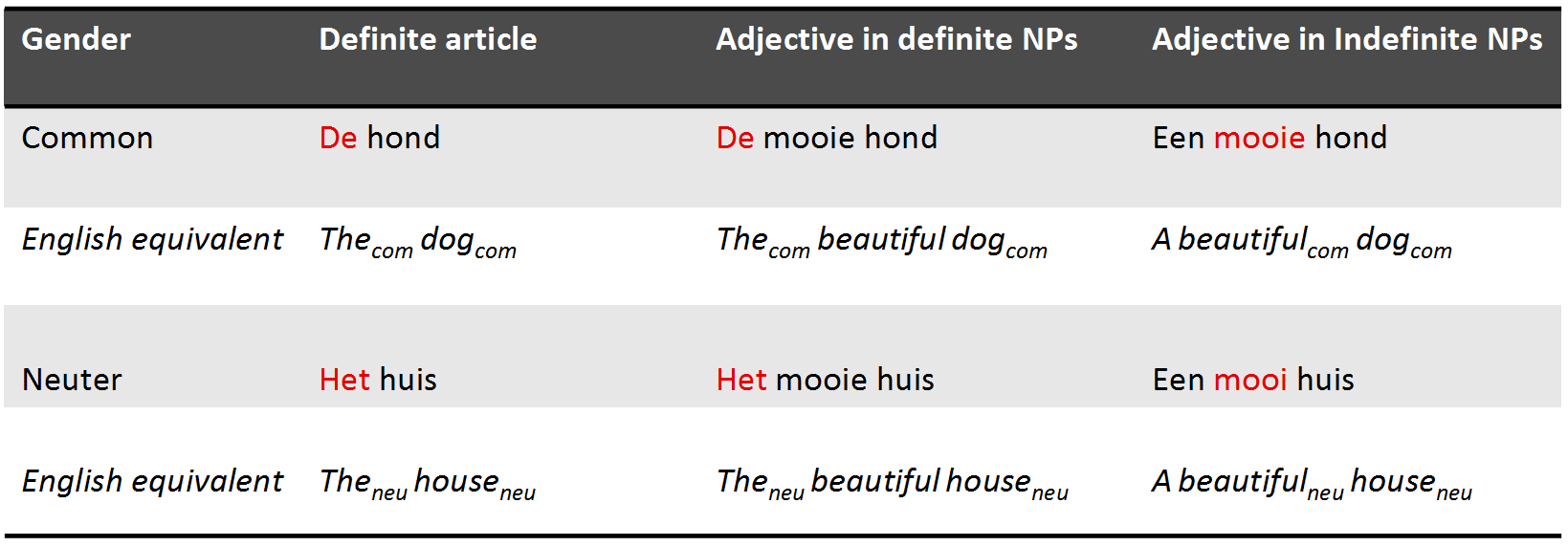
- Gender in Dutch: 70% common, 30% neuter
- When a noun is diminutive it is always neuter
- Gender is unpredictable from the root noun and hard to learn
Why use eye tracking?
- Eye tracking reveals incremental processing of the listener during time course of speech signal
- As people tend to look at what they hear (Cooper, 1974), lexical competition can be tested
Testing lexical competition using eye tracking
- Cohort Model (Marslen-Wilson & Welsh, 1978): Competition between words is based on word-initial activation
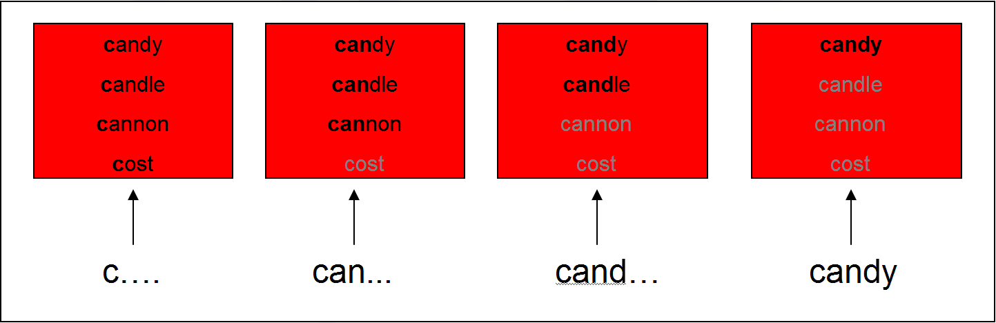
- This can be tested using the visual world paradigm: following eye movements while participants receive auditory input to click on one of several objects on a screen
Support for the Cohort Model
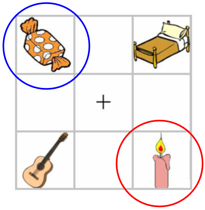
- Subjects hear: "Pick up the candy" (Tanenhaus et al., 1995)
- Fixations towards target (Candy) and competitor (Candle): support for the Cohort Model
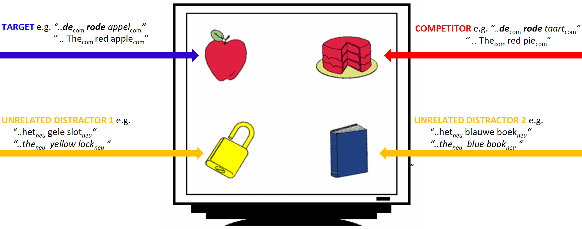
Lexical competition based on syntactic gender
- Other models of lexical processing state that lexical competition occurs based on all acoustic input (e.g., TRACE, Shortlist, NAM)
- Does gender information restrict the possible set of lexical candidates?
- If you hear de, do you focus more on a dog (de hond) than on a horse (het paard)?
- Previous studies (e.g., Dahan et al., 2000 for French) have indicated gender information restricts the possible set of lexical candidates
- We will investigate if this also holds for Dutch with its difficult gender system using the VWP
- We analyze the data using mixed-effects regression in
R
Experimental design
- 28 Dutch participants heard sentences like:
- Klik op de rode appel ('click on the red apple')
- Klik op het plaatje met een blauw boek ('click on the image of a blue book')
- They were shown 4 nouns varying in color and gender
- Eye movements were tracked with a Tobii eye-tracker (E-Prime extensions)
Experimental design: conditions
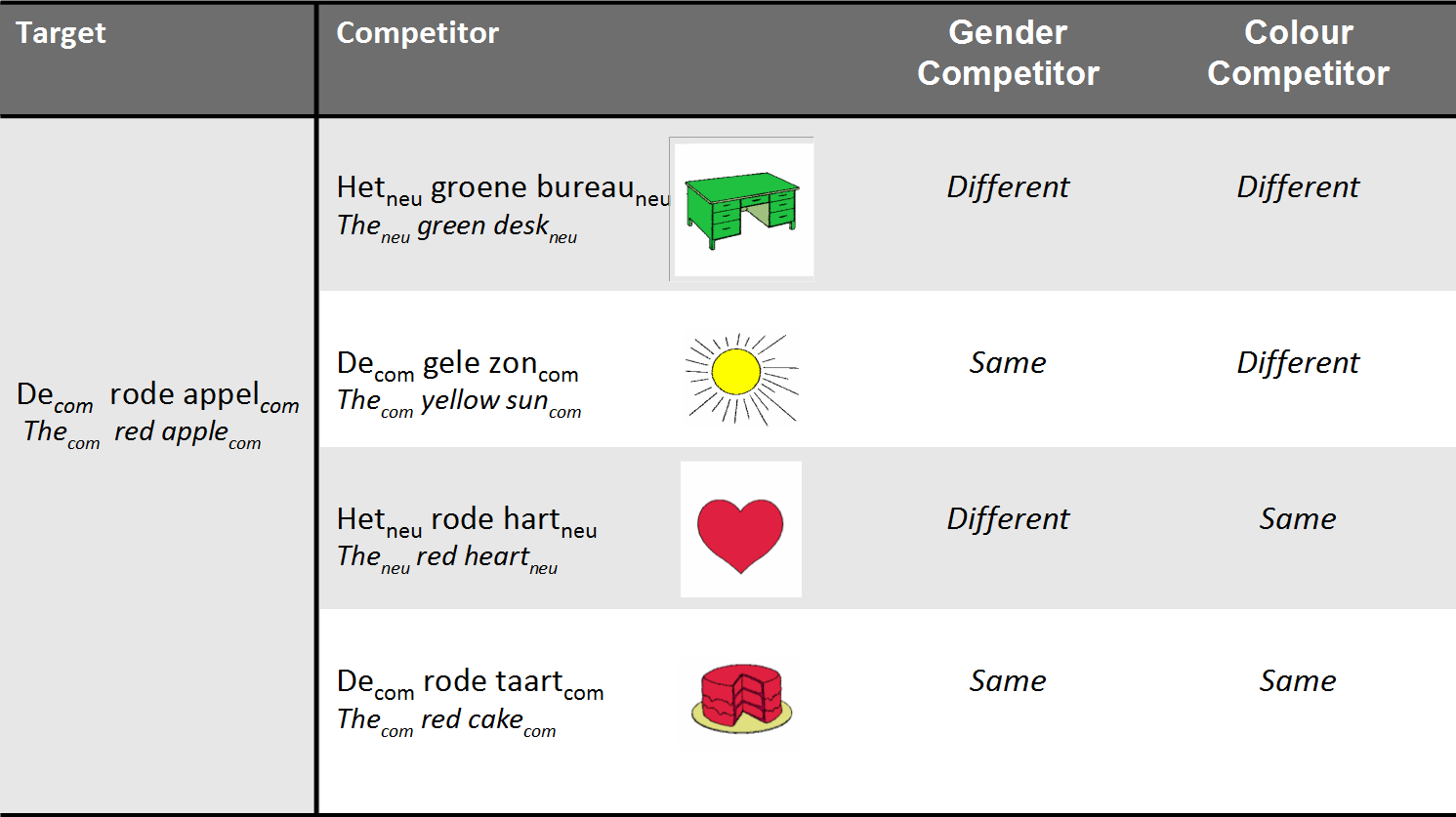
- Subjects were shown 96 different screens
- 48 screens for indefinite sentences (klik op het plaatje met een rode appel)
- 48 screens for definite sentences (klik op de rode appel)
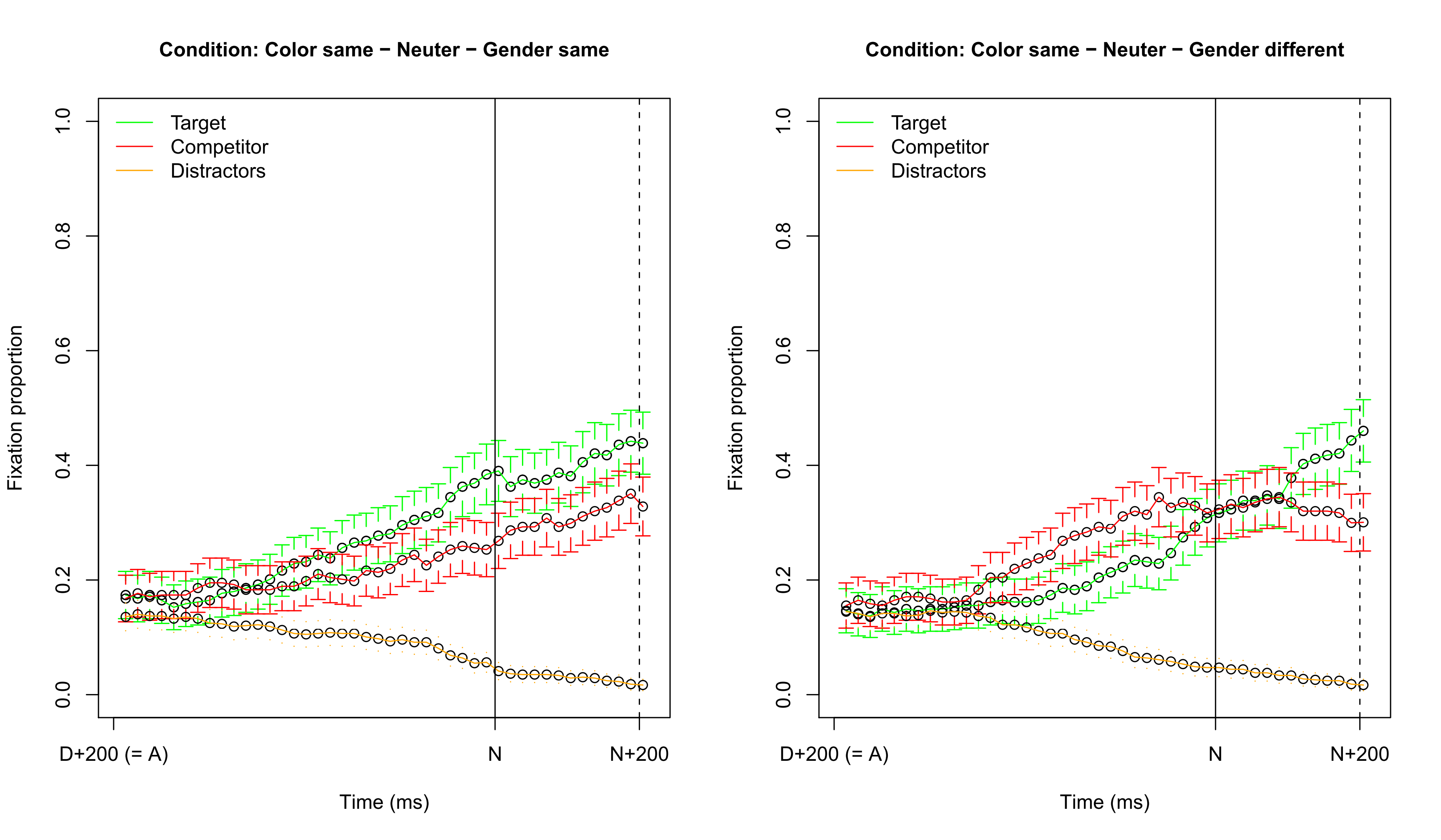
Visualizing fixation proportions: different color
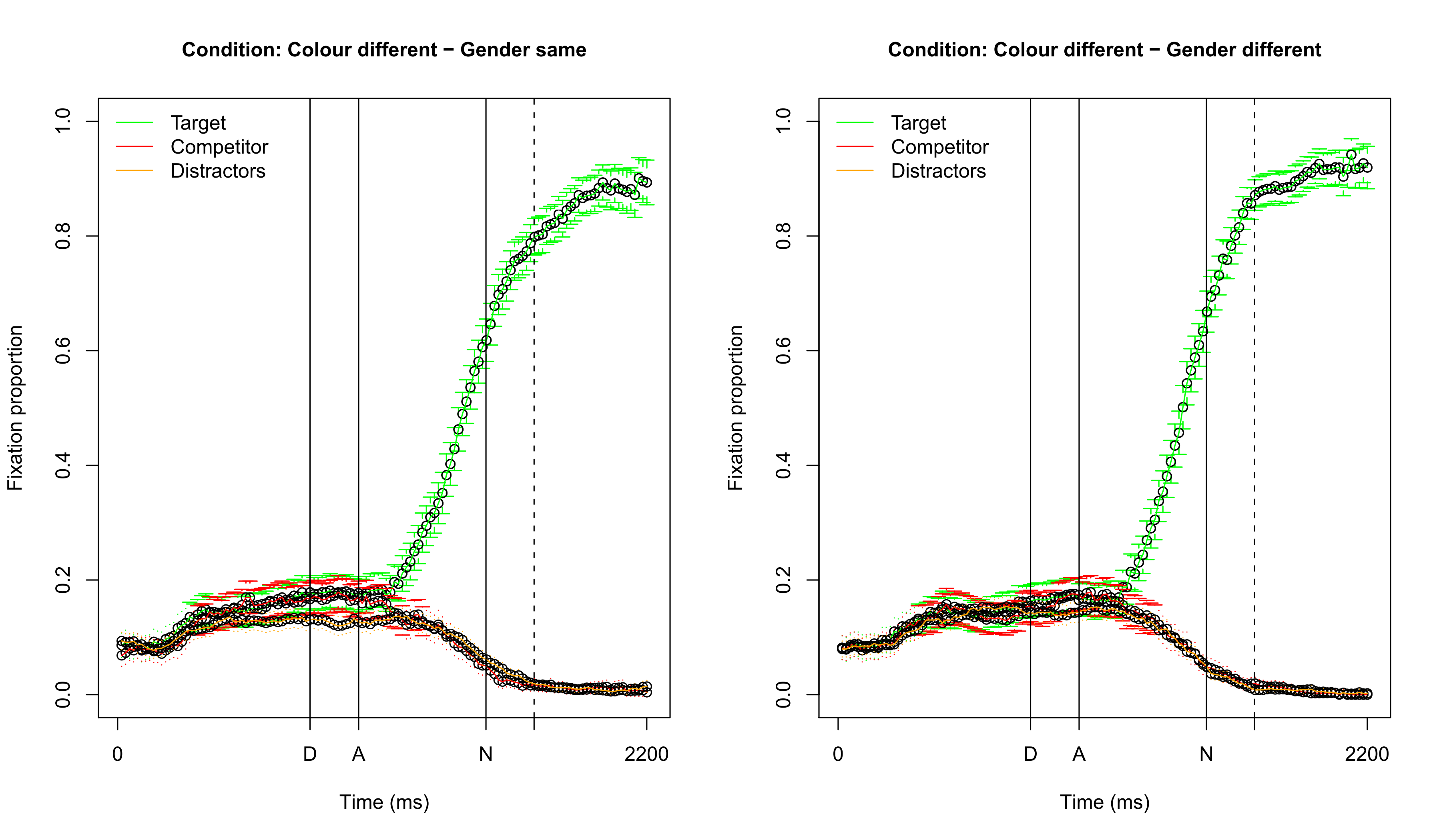
Visualizing fixation proportions: same color
Which dependent variable? (1)
- Difficulty 1: choosing the dependent variable
- Fixation difference between Target and Competitor
- Fixation proportion on Target: requires transformation to empirical logit, to ensure the dependent variable is unbounded: \(log( \frac{(y + 0.5)}{(N - y + 0.5)} )\) (or use logistic regression)
- Logistic regression comparing fixations on Target versus Competitor
- Difficulty 2: selecting a time span
- Note that about 200 ms. is needed to plan and launch an eye movement
- It is possible (and better) to take every individual sampling point into account, but we will opt for the simpler approach here (in contrast to the GAM approach explained in later lectures)
Question 1
Which dependent variable? (2)
- Here we use logistic regression comparing fixations on Target versus Competitor
- Averaged over the time span starting 200 ms. after the onset of the determiner and ending 200 ms. after the onset of the noun (about 800 ms.)
- This ensures that gender information has been heard and processed, both for the definite and indefinite sentences
Logistic regression
- Dependent variable is binary (1: success, 0: failure), not continuous
- Transform to continuous variable via log odds link function: \(\log(\frac{p}{1-p})\) = logit\((p)\)
- Done automatically in regression by setting
family="binomial"
- Done automatically in regression by setting
- Generalized linear model: specific link function and error distribution
- Interpret coefficients w.r.t. success as logits: in
R:plogis(x)
Independent variables (1)
- Variable of interest:
- Competitor gender vs. target gender
- Variables which could be important:
- Competitor color vs. target color
- Gender of target (common or neuter)
- Definiteness of target
Independent variables (2)
- Participant-related variables:
- Gender (male/female), age, education level
- Trial number
- Design control variables:
- Competitor position vs. target position (up-down or down-up)
- Color of target
- (anything else you are not interested in, but potentially problematic)
Question 2
Some remarks about data preparation
- Check if variables correlate highly
- If so: exclude variable / combine variables (residualization is not OK: Wurm & Fisicaro, 2014)
- See Chapter 6.2.2 of Baayen (2008)
- Check distribution of numerical predictors
- If skewed: it may help to try to make them normal (e.g., log. or inverse transformation)
- With logistic regression there is no normality assumption for the residuals
- Center your numerical predictors when doing mixed-effects regression
- See previous lecture
Our data
head(eye)
#   Subject   Item TargetDefinite TargetNeuter TargetColor TargetPlace CompColor CompPlace TrialID
# 1    S300   boom              1            0       green           3     brown         2       1
# 2    S300  bloem              1            0         red           4     green         2       2
# 3    S300  anker              1            1      yellow           3    yellow         2       3
# 4    S300   auto              1            0       green           3     brown         2       4
# 5    S300   boek              1            1        blue           4      blue         3       5
# 6    S300 varken              1            1       brown           1     green         3       6
#   Age IsMale Edulevel SameColor SameGender TargetFocus CompFocus
# 1  52      0        1         0          1          43        41
# 2  52      0        1         0          0         100         0
# 3  52      0        1         1          1          73        27
# 4  52      0        1         0          0         100         0
# 5  52      0        1         1          0          12        21
# 6  52      0        1         0          0           0        51
Our first generalized mixed-effects regression model
(R version 3.3.2 (2016-10-31), lme4 version 1.1.12)
library(lme4)
summary(model <- glmer(cbind(TargetFocus, CompFocus) ~ (1 | Subject) + (1 | Item), data = eye, family = "binomial"))  # intercept-only model
# Generalized linear mixed model fit by maximum likelihood (Laplace Approximation) ['glmerMod']
#  Family: binomial  ( logit )
# Formula: cbind(TargetFocus, CompFocus) ~ (1 | Subject) + (1 | Item)
#    Data: eye
#
#      AIC      BIC   logLik deviance df.resid
#   125387   125404   -62690   125381     2263
#
# Scaled residuals:
#    Min     1Q Median     3Q    Max
# -42.14  -4.12   2.37   5.17  11.40
#
# Random effects:
#  Groups  Name        Variance Std.Dev.
#  Item    (Intercept) 0.106    0.326
#  Subject (Intercept) 0.345    0.588
# Number of obs: 2266, groups:  Item, 48; Subject, 28
#
# Fixed effects:
#             Estimate Std. Error z value Pr(>|z|)
# (Intercept)    0.848      0.121    7.02  2.3e-12 ***
# ---
# Signif. codes:  0 '***' 0.001 '**' 0.01 '*' 0.05 '.' 0.1 ' ' 1
By-item random intercepts

By-subject random intercepts

Interpreting logit coefficients I
summary(model)$coef
#             Estimate Std. Error z value Pr(>|z|)
# (Intercept)    0.848      0.121    7.02 2.28e-12
plogis(fixef(model)["(Intercept)"])
# (Intercept)
#         0.7
- On average 70% chance to focus on target

Is a by-item analysis necessary?
# In the Gaussian case, the REML parameter needs to be set to TRUE when comparing models only
# differing in the random effects; For glmer, this parameter is absent, as it only allows ML fitting.
model1 <- glmer(cbind(TargetFocus, CompFocus) ~ (1 | Subject), data = eye, family = "binomial")
model2 <- glmer(cbind(TargetFocus, CompFocus) ~ (1 | Subject) + (1 | Item), data = eye, family = "binomial")
AIC(model1) - AIC(model2)
# [1] 2917
- The AIC difference is much higher than 2, so we include the by-item random intercept
Adding a fixed-effect factor
model3 <- glmer(cbind(TargetFocus, CompFocus) ~ SameColor + (1 | Subject) + (1 | Item), data = eye, family = "binomial")
summary(model3)$coef
#             Estimate Std. Error z value Pr(>|z|)
# (Intercept)     1.68     0.1209    13.9 7.44e-44
# SameColor      -1.48     0.0118  -125.5 0.00e+00
SameColoris highly significant- Negative estimate: less likely to focus on target
- We need to test if the effect of
SameColorvaries per subject - If there is much between-subject variation, this will influence variable signficance
Testing for a random slope
model4 <- glmer(cbind(TargetFocus, CompFocus) ~ SameColor + (1 + SameColor | Subject) + (1 | Item), data = eye,
    family = "binomial")  # the random slope SameColor needs to be correlated with the random intercept
AIC(model3) - AIC(model4)
# [1] 2218
summary(model4)$varcor
#  Groups  Name        Std.Dev. Corr
#  Item    (Intercept) 0.359
#  Subject (Intercept) 1.251
#          SameColor   0.949    -0.95
summary(model4)$coef
#             Estimate Std. Error z value Pr(>|z|)
# (Intercept)     1.89      0.245     7.7 1.36e-14
# SameColor      -1.71      0.184    -9.3 1.40e-20
- Note
SameColoris still highly significant
Investigating the gender effect
model5 <- glmer(cbind(TargetFocus, CompFocus) ~ SameColor + SameGender + (1 + SameColor | Subject) +
    (1 | Item), data = eye, family = "binomial")
summary(model5)$coef
#             Estimate Std. Error z value Pr(>|z|)
# (Intercept)   1.8536     0.2462    7.53 5.08e-14
# SameColor    -1.7124     0.1846   -9.28 1.74e-20
# SameGender    0.0742     0.0115    6.47 9.97e-11
- It seems the gender is effect is opposite to our expectations...
- Perhaps there is an effect of common vs. neuter gender?
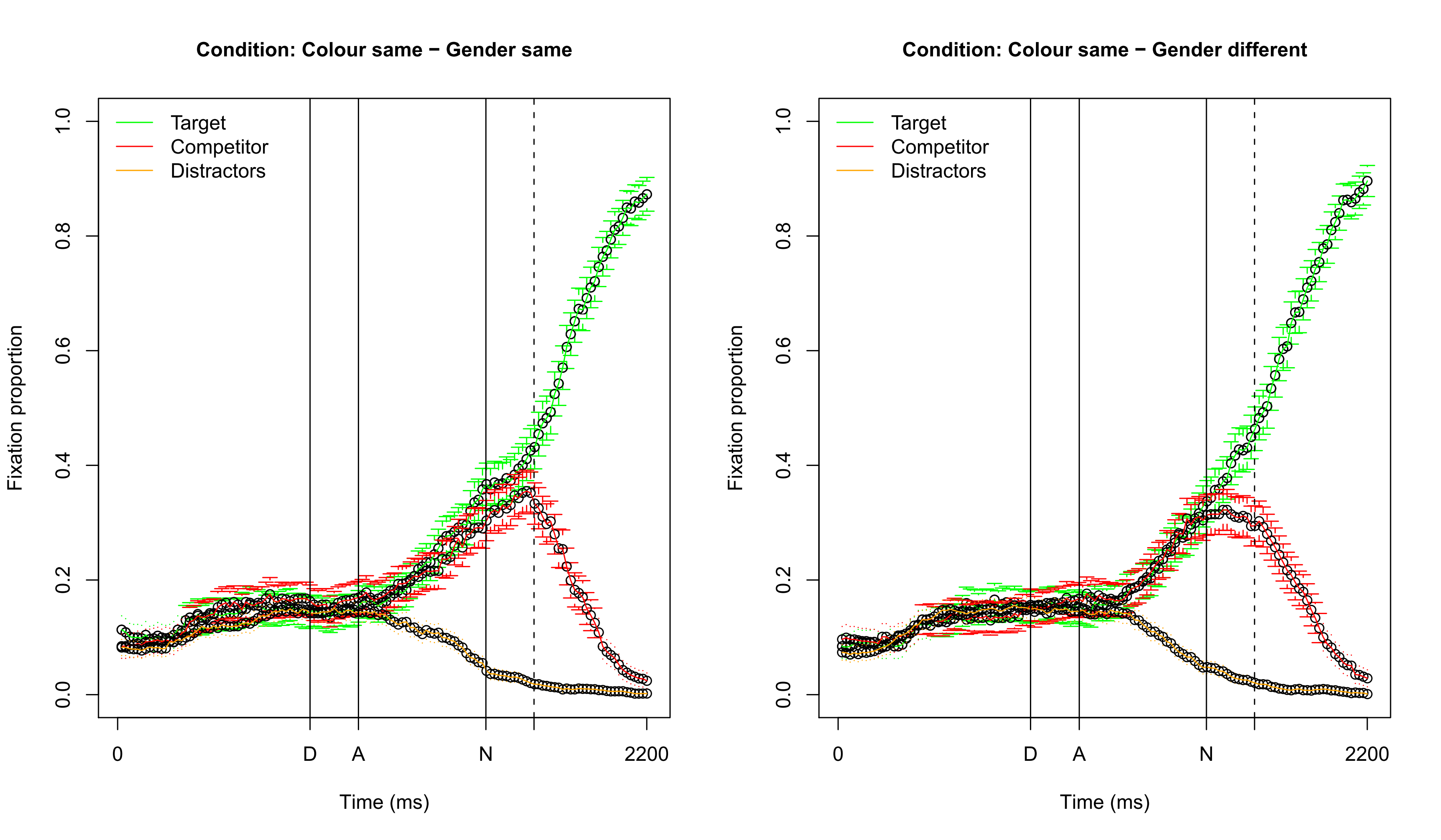
Visualizing fixation proportions: target common
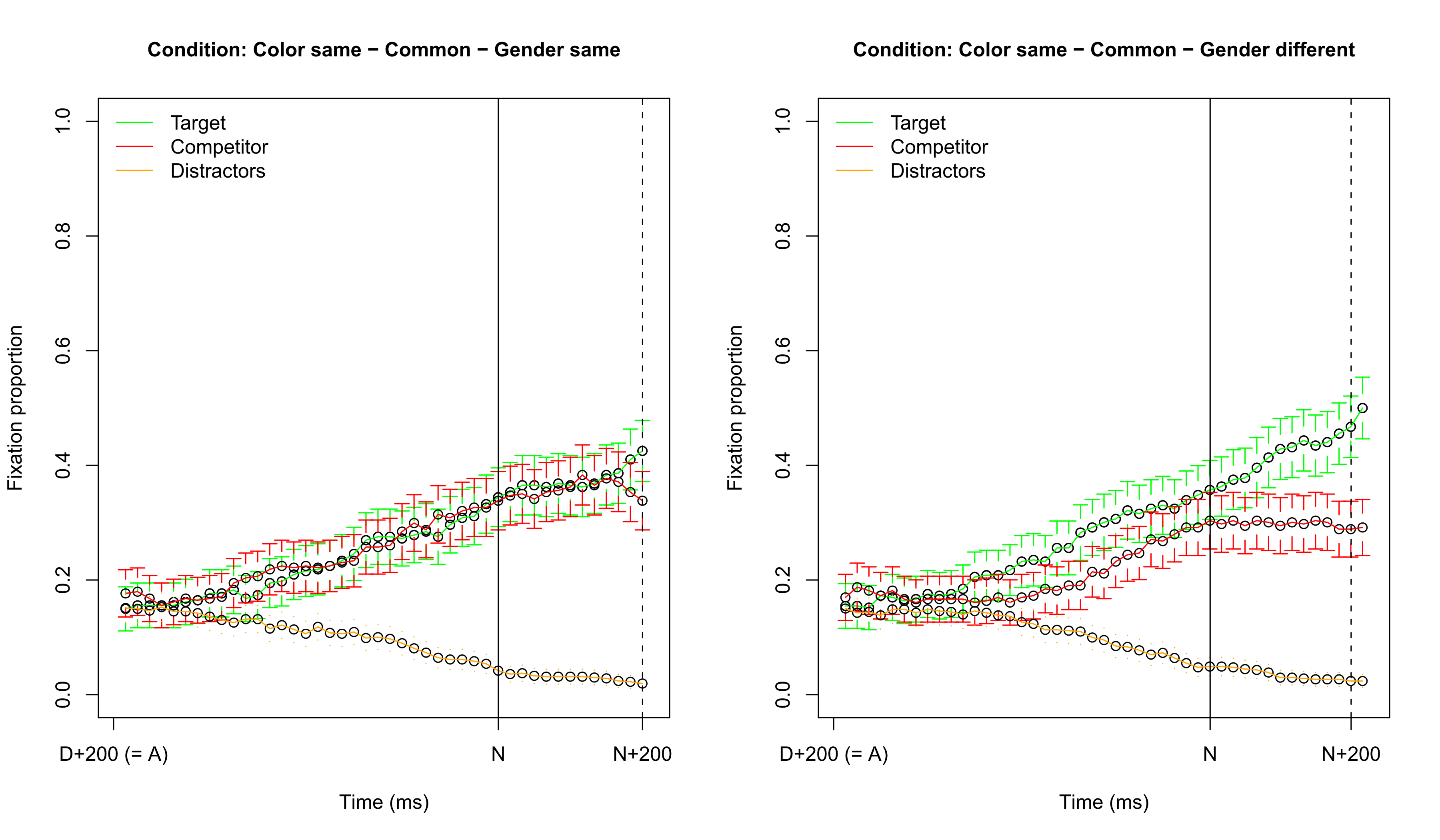
Visualizing fixation proportions: target neuter
No simple influence of common vs. neuter
model6 <- glmer(cbind(TargetFocus, CompFocus) ~ SameColor + SameGender + TargetNeuter + (1 + SameColor |
    Subject) + (1 | Item), data = eye, family = "binomial")
summary(model6)$coef
#              Estimate Std. Error z value Pr(>|z|)
# (Intercept)    1.9398     0.2509    7.73 1.06e-14
# SameColor     -1.7125     0.1845   -9.28 1.65e-20
# SameGender     0.0742     0.0115    6.47 9.92e-11
# TargetNeuter  -0.1723     0.1015   -1.70 8.96e-02
Testing the interaction
model7 <- glmer(cbind(TargetFocus, CompFocus) ~ SameColor + SameGender * TargetNeuter + (1 + SameColor |
    Subject) + (1 | Item), data = eye, family = "binomial")
summary(model7)$coef
#                         Estimate Std. Error z value  Pr(>|z|)
# (Intercept)                2.067     0.2512    8.23  1.88e-16
# SameColor                 -1.716     0.1846   -9.30  1.43e-20
# SameGender                -0.174     0.0164  -10.63  2.27e-26
# TargetNeuter              -0.416     0.1026   -4.05  5.13e-05
# SameGender:TargetNeuter    0.488     0.0230   21.24 4.35e-100
- There is clear support for an interaction
- These results are in line with the previous fixation proportion graphs
Testing if the interaction yields an improved model
# As glmer has only a single fitting option (ML), we can immediately compare model7 (SameColor +
# SameGender * TargetNeuter) to the best previous model model5 (SameColor + SameGender)
AIC(model5) - AIC(model7)
# [1] 451
- The interaction improves the model significantly
- Unfortunately, we do not have an explanation for the strange neuter pattern
- Note that we still need to test the variables for inclusion as random slopes (in lab session)
Adding a factor to the model
# set a reference level for the factor
eye$TargetColor <- relevel(eye$TargetColor, "brown")
model8 <- glmer(cbind(TargetFocus, CompFocus) ~ SameColor + SameGender * TargetNeuter + TargetColor +
    (1 + SameColor | Subject) + (1 | Item), data = eye, family = "binomial")
summary(model8)$coef
#                         Estimate Std. Error z value  Pr(>|z|)
# (Intercept)                1.707     0.2672    6.39  1.65e-10
# SameColor                 -1.717     0.1848   -9.29  1.59e-20
# SameGender                -0.174     0.0164  -10.63  2.16e-26
# TargetNeuter              -0.415     0.0880   -4.72  2.32e-06
# TargetColorblue            0.275     0.1433    1.92  5.50e-02
# TargetColorgreen           0.494     0.1435    3.44  5.78e-04
# TargetColorred             0.456     0.1434    3.18  1.47e-03
# TargetColoryellow          0.502     0.1434    3.50  4.67e-04
# SameGender:TargetNeuter    0.488     0.0230   21.24 3.76e-100
Comparing different factor levels
library(multcomp)
summary(glht(model8, linfct = mcp(TargetColor = "Tukey")))
#
#    Simultaneous Tests for General Linear Hypotheses
#
# Multiple Comparisons of Means: Tukey Contrasts
#
#
# Fit: glmer(formula = cbind(TargetFocus, CompFocus) ~ SameColor + SameGender *
#     TargetNeuter + TargetColor + (1 + SameColor | Subject) +
#     (1 | Item), data = eye, family = "binomial")
#
# Linear Hypotheses:
#                     Estimate Std. Error z value Pr(>|z|)
# blue - brown == 0    0.27510    0.14335    1.92   0.3067
# green - brown == 0   0.49375    0.14346    3.44   0.0051 **
# red - brown == 0     0.45611    0.14338    3.18   0.0129 *
# yellow - brown == 0  0.50161    0.14335    3.50   0.0042 **
# green - blue == 0    0.21865    0.13518    1.62   0.4857
# red - blue == 0      0.18101    0.13508    1.34   0.6657
# yellow - blue == 0   0.22651    0.13507    1.68   0.4479
# red - green == 0    -0.03764    0.13518   -0.28   0.9987
# yellow - green == 0  0.00786    0.13517    0.06   1.0000
# yellow - red == 0    0.04550    0.13507    0.34   0.9972
# ---
# Signif. codes:  0 '***' 0.001 '**' 0.01 '*' 0.05 '.' 0.1 ' ' 1
# (Adjusted p values reported -- single-step method)
Simplifying the factor in a contrast
eye$TargetBrown <- (eye$TargetColor == "brown") * 1
model9 <- glmer(cbind(TargetFocus, CompFocus) ~ SameColor + SameGender * TargetNeuter + TargetBrown +
    (1 + SameColor | Subject) + (1 | Item), data = eye, family = "binomial")
summary(model9)$coef
#                         Estimate Std. Error z value  Pr(>|z|)
# (Intercept)                2.139     0.2502    8.55  1.23e-17
# SameColor                 -1.717     0.1849   -9.28  1.62e-20
# SameGender                -0.174     0.0164  -10.63  2.14e-26
# TargetNeuter              -0.415     0.0913   -4.55  5.36e-06
# TargetBrown               -0.432     0.1215   -3.55  3.82e-04
# SameGender:TargetNeuter    0.488     0.0230   21.24 3.96e-100
AIC(model9) - AIC(model8) # N.B. model8 is more complex
# [1] -2.43
Interpreting logit coefficients II
# chance to focus on target
# when there is a color
# competitor and a gender
# competitor, while the target
# is common and not brown
(logit <- fixef(model9)["(Intercept)"] +
    1 * fixef(model9)["SameColor"] +
    1 * fixef(model9)["SameGender"] +
    0 * fixef(model9)["TargetNeuter"] +
    0 * fixef(model9)["TargetBrown"] +
    1 * 0 * fixef(model9)["SameGender:TargetNeuter"])
# (Intercept)
#       0.248
plogis(logit) # was 0.7
# (Intercept)
#       0.562

Distribution of residuals
qqnorm(resid(model9))
qqline(resid(model9))

- Not normal, but also not required for logistic regression!
Model criticism
eye2 <- eye[abs(scale(resid(model9))) < 2.5, ]  # remove items with which the model has trouble fitting
1 - (nrow(eye2)/nrow(eye))  # only about 0.5% removed
# [1] 0.0053
model10 <- glmer(cbind(TargetFocus, CompFocus) ~ SameColor + SameGender * TargetNeuter + TargetBrown +
    (1 + SameColor | Subject) + (1 | Item), data = eye2, family = "binomial")
summary(model10)$coef  # all variables significant
#                         Estimate Std. Error z value  Pr(>|z|)
# (Intercept)                2.292     0.2981    7.69  1.51e-14
# SameColor                 -1.782     0.1953   -9.12  7.27e-20
# SameGender                -0.213     0.0166  -12.85  8.15e-38
# TargetNeuter              -0.419     0.0984   -4.26  2.07e-05
# TargetBrown               -0.460     0.1311   -3.51  4.48e-04
# SameGender:TargetNeuter    0.562     0.0233   24.13 1.16e-128
Question 3
Many more things to do...
- We still need to:
- See if the significant fixed effects remain significant when adding the (necessary) by-subject random slopes
- See if there are other variables we should test (e.g., education level)
- See if there are other interactions we can test
- Apply model criticism after these steps
- We will experiment with these points in the lab session after the break!
- We use a subset of the data (only same color)
- Simple
R-functions are used to generate all plots
Recap
- We have learned how to create logistic mixed-effects regression models
- We have learned that mixed-effects regression models:
- Are useful when your design is not completely balanced
- Allow a detailed inspection of the variability of the random effects for additional insight
- Note that we analyzed this data in a non-optimal way:
- It would be better to predict the focus for every individual timepoint
- After the break:
- Next lecture: introduction to generalized additive modeling
Evaluation
Questions?
Thank you for your attention!