I follow the construction defined by [32] to
extend ![]() , giving
, giving
![]() (
(![]() ), by adding a set of relation symbols
), by adding a set of relation symbols
![]() , conjunction, negation and existential quantification. The
syntax I use for these will be clear from the definition of the
interpretations of
, conjunction, negation and existential quantification. The
syntax I use for these will be clear from the definition of the
interpretations of
![]() (
(![]() ) (essentially Prolog syntax where
appropriate).
) (essentially Prolog syntax where
appropriate).
The interpretation ![]() of
of
![]() (
(![]() ) is defined in terms of the
interpretation
) is defined in terms of the
interpretation ![]() of
of ![]() . The expression
. The expression
![]() [s
[s ![]() X] defines the assignment which is exactly like
X] defines the assignment which is exactly like ![]() ,
except possibly for the variable X which gets assigned the element
s. An interpretation
,
except possibly for the variable X which gets assigned the element
s. An interpretation ![]() of
of
![]() (
(![]() ) is obtained from
) is obtained from ![]() (
(![]() is said to be based on
is said to be based on ![]() ) by choosing for every
relation symbol
r
) by choosing for every
relation symbol
r ![]()
![]() a relation
r
a relation
r![]() on
on
![]()
![]() taking the right number of arguments. Furthermore, let
taking the right number of arguments. Furthermore, let
Implication, universal quantification and disjunction may be defined
in terms of these connectives. The formalism consists of
definite clauses of
![]() (
(![]() ). I write such a definite clause as:
). I write such a definite clause as:
![]()
where
p,q1...qn are atoms and ![]() is a
is a
![]() constraint. Atoms look as
r(X1,...,Xn)
where
r
constraint. Atoms look as
r(X1,...,Xn)
where
r ![]() R and
X1...Xn
R and
X1...Xn ![]() V.
V.
A partial order on the set of all
![]() (
(![]() ) interpretations is defined
as follows:
) interpretations is defined
as follows:
![]()
![]()
![]() iff for all
r
iff for all
r ![]() R,r
R,r![]()
![]() r
r![]() . The union of a set of
. The union of a set of
![]() (
(![]() )
interpretations is obtained by joining the denotations of the relation
symbols and is again an
)
interpretations is obtained by joining the denotations of the relation
symbols and is again an
![]() (
(![]() ) interpretation. A model M of a set
of definite clauses
) interpretation. A model M of a set
of definite clauses ![]() is defined as an
is defined as an
![]() (
(![]() ) interpretation such that
M satisfies
) interpretation such that
M satisfies ![]() , i.e.,
, i.e.,
![]() M = ASSM.
M = ASSM.
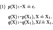
The use of definite clauses is motivated by the following theorem, proven in [32] for the general case.
![]()
![]()
This defines a chain
![]() 0
0 ![]()
![]() 1
1 ![]() ...
of
...
of
![]() (
(![]() ) interpretations, based on
) interpretations, based on ![]() . Moreover, the union
. Moreover, the union
![]()
is the least model of ![]() extending
extending ![]() .
.
This theorem says that if ![]() is a set of definite clauses, then
is a set of definite clauses, then
![]() uniquely defines the relations of
uniquely defines the relations of ![]() ; i.e.
; i.e. ![]() defines unique minimal denotations for the relation symbols of
defines unique minimal denotations for the relation symbols of ![]() .
.
Clearly,
p![]() 0 and
q
0 and
q![]() 0 are both the empty set.
Because the assignments are based on
0 are both the empty set.
Because the assignments are based on ![]() we know the solutions of
the constraints. Therefore, we obtain
we know the solutions of
the constraints. Therefore, we obtain
| p |
= | { |
|
| = | { |
||
| = | { |
||
| = | {(c, |
| q |
= | { |
|
| = | { |
||
| = | { |
||
| = | {(c, |
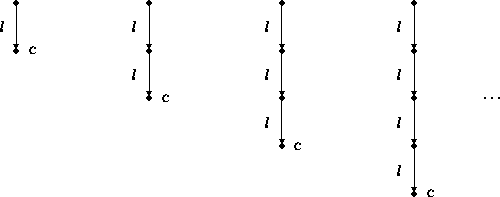
| 0 | 1 | 2 | 3 | 4 | 5 | ... | |
| p | { c} | { c} | { c} | { c} | { c} | ... | |
| q | { c} | { c, f1} | { c, f1, f2} | { c, f1, f2, f3} | ... |
A goal or query is a possibly empty conjunction of
![]() (
(![]() )-atoms and a
)-atoms and a ![]() -constraint, written as:
-constraint, written as:
![]()
An answer to a goal is a satisfiable constraint ![]() , such
that
, such
that
![]()
![]() p1...pn,
p1...pn,![]() is valid
(given a set of clauses
is valid
(given a set of clauses ![]() ) in the minimal model of
) in the minimal model of ![]() .
For example, for the previous definite clause program a possible
answer to the goal
.
For example, for the previous definite clause program a possible
answer to the goal
![]()
is the answer:
![]()
because
X0l ![]() c
c ![]() q(X0) is valid in the minimal model.
q(X0) is valid in the minimal model.