 |
 |
In both of these definitions, the number of transitions should be understood as the the number of non-duplicate transitions which do not lead to a sink state. A sink state is a state from which there exists no sequence of transitions to a final state. In the randomly generated automata, states are accessible and co-accessible by construction; sink states and associated transitions are not represented.
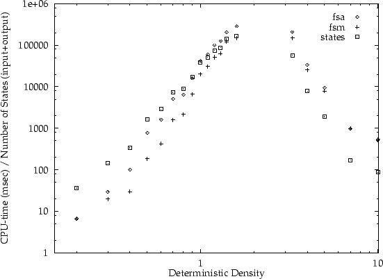
[11] shows that deterministic transition density is a reliable measure for the difficulty of subset construction. Exponential blow-up can be expected for input automata with deterministic transition density of around 2.6 He concludes (page 66):
[...] randomly generated automata exhibit the maximum execution time, and the maximum number of states, at an approximate deterministic density of 2. Most of the area under the curve occurs within 0.5 and 2.5 deterministic density--this is the area in which subset construction is expensive.
Conjecture. For a given NFA, we can compute the expected numbers of states and transitions in the corresponding DFA, produced by subset construction, from the deterministic density of the NFA. In addition, this functional relationship gives rise to a Poisson-like curve with its peak approximately at a deterministic density of 2.
A number of automata were generated randomly, according to the number
of states, symbols, and transition density. For the first experiment,
automata were generated consisting of 15 symbols, 25 states, and
various densities (and no ![]() -moves). The results are
summarised in figure 5. CPU-time was measured on a HP
9000/785 machine running HP-UX 10.20. Note that our timings do not
include the start-up of the Prolog engine, nor the time required for
garbage collection.
-moves). The results are
summarised in figure 5. CPU-time was measured on a HP
9000/785 machine running HP-UX 10.20. Note that our timings do not
include the start-up of the Prolog engine, nor the time required for
garbage collection.
In order to establish that the differences we obtain later are
genuinely due to differences in the underlying algorithm, and not due
to `accidental' implementation details, we have compared our
implementation with the determiniser of AT&T's FSM utilities
[13]. For automata without ![]() -moves we establish
that FSM normally is faster: for automata with very small transition
densities FSM is up to four times as fast, for automata with larger
densities the results are similar.
-moves we establish
that FSM normally is faster: for automata with very small transition
densities FSM is up to four times as fast, for automata with larger
densities the results are similar.
A new concept called absolute jump density is introduced to
specify the number of ![]() -moves. It is defined as the number of
-moves. It is defined as the number of
![]() -moves divided by the square of the number of states (i.e.,
the probability that an
-moves divided by the square of the number of states (i.e.,
the probability that an ![]() -move exists for a given pair of
states). Furthermore, deterministic jump density is the
number of
-move exists for a given pair of
states). Furthermore, deterministic jump density is the
number of ![]() -moves divided by the number of states (i.e., the
average number of
-moves divided by the number of states (i.e., the
average number of ![]() -moves which leave a given state). In
order to measure the differences between the three implementations, a
number of automata has been generated consisting of 15 states and 15
symbols, using various transition densities between 0.01 and 0.3 (for
larger densities the automata tend to collapse to an automaton for
-moves which leave a given state). In
order to measure the differences between the three implementations, a
number of automata has been generated consisting of 15 states and 15
symbols, using various transition densities between 0.01 and 0.3 (for
larger densities the automata tend to collapse to an automaton for
![]() ). For each of these transition densities, deterministic
jump densities were chosen in the range 0 to 2.5 (again, for larger
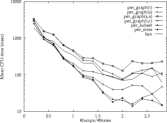
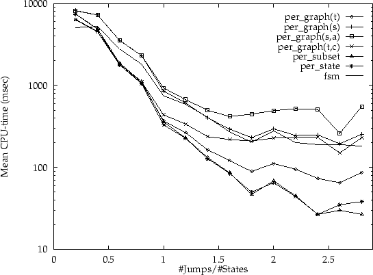
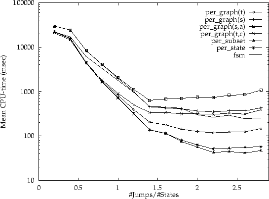
values the automata tend to collapse). In figures 6 to
9 the outcomes of these experiments are summarised by
listing the average amount of CPU-time required per deterministic jump
density (for each of the algorithms), using automata with 15, 20, 25
and 100 states respectively. Thus, every dot represents
the average for determinising a number of different input automata
with various absolute transition densities and the same deterministic
jump density.
). For each of these transition densities, deterministic
jump densities were chosen in the range 0 to 2.5 (again, for larger
values the automata tend to collapse). In figures 6 to
9 the outcomes of these experiments are summarised by
listing the average amount of CPU-time required per deterministic jump
density (for each of the algorithms), using automata with 15, 20, 25
and 100 states respectively. Thus, every dot represents
the average for determinising a number of different input automata
with various absolute transition densities and the same deterministic
jump density.
 |
 |
 |
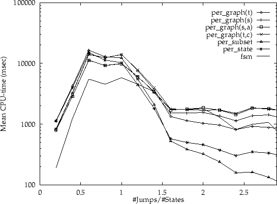 |
The striking aspect of these experiments is that the integrated per subset and per state variants are much more efficient for larger deterministic jump density. The per grapht is typically the fastest algorithm of the non-integrated versions. However, in these experiments all states in the input are co-accessible by construction; and moreover, all states in the input are final states. Therefore, the advantages of the per grapht,c algorithm could not be observed here.
The turning point is around a deterministic jump density of around 0.8: for smaller densities the per grapht is typically slightly faster; for larger densities the per state algorithm is much faster. For densities beyond 1.5, the per subset algorithm tends to perform better than the per state algorithm. Interestingly, this generalisation is supported by the experiments on automata which were generated by approximation techniques (although the results for randomly generated automata are more consistent than the results for `real' examples).