An interpretation ![]() of
of ![]() consists of a domain
D
consists of a domain
D![]() which is the set of all feature graphs built from L, C and V,
and a solution mapping
.
which is the set of all feature graphs built from L, C and V,
and a solution mapping
. ![]() which will be defined below.
An
which will be defined below.
An ![]() -assignment is a mapping from the set of variables to
D
-assignment is a mapping from the set of variables to
D![]() . I write
ASS
. I write
ASS![]() for the set of all
for the set of all
![]() -assignments. Variables and constants will denote feature graphs,
relative to some assignment.
-assignments. Variables and constants will denote feature graphs,
relative to some assignment.
The denotation of a variable
X w.r.t. assignment ![]() is
simply
is
simply
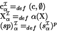
![]() (X). The denotation of a constant
c is the
feature graph
(c,
(X). The denotation of a constant
c is the
feature graph
(c,![]() ) (for any assignment). The denotation of
a descriptor sp is defined as Fp where F is the
denotation of s; i.e. the denotation of sp is the subgraph
at p of the graph denoted by s. Note that the denotation of some
descriptors is undefined. Summarizing:
) (for any assignment). The denotation of
a descriptor sp is defined as Fp where F is the
denotation of s; i.e. the denotation of sp is the subgraph
at p of the graph denoted by s. Note that the denotation of some
descriptors is undefined. Summarizing:
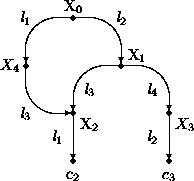
As an example, consider the feature graph F2 in figure 2.2.
For an assignment that maps X to the feature graph F2, the denotation of the descriptor Xl1l3 is the subgraph rooted at X2. Similarly, the denotation of Xl2l4l2 is the feature graph (c3,
An interpretation ![]() satisfies an atomic constraint
satisfies an atomic constraint
![]() = d1
= d1 ![]() d2, relative to an assignment
d2, relative to an assignment ![]() , written
, written
![]()
![]()
![]() if the denotation of descriptors d1, d2
are both defined and the same, i.e.:
if the denotation of descriptors d1, d2
are both defined and the same, i.e.:
![]()
Hence, ![]() satisfies the equation
Xl1l3
satisfies the equation
Xl1l3 ![]() Xl2l3 with respect to the assignment that maps X to
the feature graph F2 defined above. As another example,
Xl2l3 with respect to the assignment that maps X to
the feature graph F2 defined above. As another example, ![]() also satisfies the equation
Xl1l3l1
also satisfies the equation
Xl1l3l1 ![]() c2, with the same
c2, with the same ![]() .
.
The solutions of a constraint are all assignments that give
satisfaction. Constraints are thus seen as restrictions on the values
the variables in the constraints can take. The solutions of an atomic
constraint ![]() are defined as follows:
are defined as follows:
![]()
The set of solutions of a constraint
![]() ,...,
,...,![]() is defined as
the intersection of the solutions of its atomic constraints:
is defined as
the intersection of the solutions of its atomic constraints:
A constraint is satisfiable iff it has at least one solution.
Two constraints are equivalent iff they have the same solutions.
A constraint is valid iff its solutions are all possible
assignments
ASS![]() .
.